Let me tell you a story - perhaps a familiar one.

Product Manager: Hey {data_analyst}, I looked at your dashboard! We only kicked off {AB_test_name} a few days ago, but the results look amazing! It looks like the result is already statistically significant, even though we were going to run it for another week.

Data Analyst: Absolutely, it’s very promising!

Product Manager: Well, that settles it, we can turn off the test, it looks like a winner.

Data Analyst: Woah, hold on now - we can’t do that!

Product Manager: But…why not? Your own dashboard says it’s statistically significant! Isn’t that what it’s for? Aren’t we like…95% sure, or something?

Data Analyst: Yes, but we said we would collect two weeks of data when we designed the experiment, and the analysis is only valid if we do that. I have to respect the arcane mystic powers of ✨S T A T I S T I C S✨!!!

Has this ever happened to you?

If you’re a working data scientist (or PM), it probably has. This is an example of early stopping, or optional stopping, or data peeking - and we are often cautioned to avoid it. The most frustrating part about this conversation is that it happens even when both parties are trying to be collaborative and play by the rules.

From the data scientist’s point of view, they did a power analysis and figured out how to make sure the experiment is as informative as possible. Can’t we just stick to the plan?

From the PM’s point of view, the dashboard is telling them that statistical analysis sanctions the result they see. We gave each experiment arm a chance, and one of them was the winner using their usual statistical process. Why should we wait for the full sample if an easy win is right in front of us?

The PM’s argument, frankly, makes a lot of sense. A couple more detailed arguments in favor of stopping early might look like this:

• If we think that one of the treatment groups really is better, then collecting more data is an unnecessary waste. Collecting data isn’t usually free - so it’s best to stop as soon as you can.
• If we think that one of the treatment groups really is better, than we should make it available to a larger population as soon as we can. This is not always just a question of a small gain, or a few more dollars. In clinical trials, the stakes can be very literally life or death - the trials of the HIV drug AZT were stopped short for this reason, as the results were so overwhelmingly positive that it seemed unethical to continue depriving the control group and other patients of the chance at an effective therapy. The trial was ended early and the FDA voted to approve its use shortly after (there are also more complicated factors involved in that RCT, but that’s another conversation).

The core issue here comes from the fact that good experimentation needs to balance speed vs risk. On the one hand, we want to learn and act as quick as we can. On the other, we want to avoid unnecessary risk - every experiment includes the possibility of a downside, but we want to be careful and not take on more risk than we need to.

All the possible experimentation procedures sit somewhere on this high speed-low risk tradeoff spectrum. The “highest speed” solution would be to avoid experimentation at all - just act as quick as you can. The “lowest risk” solution would be to run the experiment as planned, and always run it by the book, no matter what happens.

As is so often the case, there is a chance to get the both of worlds by picking a solution between the extremes. There are good reasons to stop a test early, but in order to do so safely, we need to be more careful about our process. Let’s start by looking at the risks of stopping early without changing our process, and then we’ll talk about how to mitigate those risks.

What risk do we take by stopping as soon as the result is significant?

Let’s remind ourselves why we do statistical significance calculations in the first place. We use P-values, confidence intervals, and all of those kinds of other frequentist devices is because they control uncertainty. The result of designing an experiment, picking a sample size based on 80% power and doing your calculations with $\alpha = 5\%$ is that the arcane mystic powers of statistics will prevent you from making a Type I error 95% of the time and a Type II error 80% of the time.

Talking about the benefits in terms of “Type I” and “Type II” errors is a little opaque. What does this do for us here in real life? We can make it concrete by talking about a more specific analysis. Let’s talk about an analysis which is very common in practice - comparing the means of two samples experimentally with a T-test. A T-test based experiment usually looks something like this:

• Pick your desired power and significant levels, usually denoted by the magic symbols $\beta$ and $\alpha$. We often use $\beta = 80\%$ and $\alpha = 5\%$, though you may pick other values based on the context.
• Use your favorite power calculator to pick a sample size, which we’ll call $n$.
• Collect $n$ samples from the control and treatment arms, and compute the difference in means $\hat{\Delta} = \overline{y^T} - \overline{y^C}$. That’s just the mean of the treated units, minus the mean of the control units.
• Use your favorite implementation of the T-test (like the one in scipy) to compute a P-value. If $p \leq \alpha$, then you can conclude that $\Delta \neq 0$, and so the treatment and control groups have different population means. Assuming the differences goes in the direction of better outcomes, you officially pop the champage and conclude that your treatment had some non-zero effect compared to control. Nice!

This procedure is a test run “by the book”, in which we collected all our data and ran a single T-test to see what happened. It guarantees that we get the usual magic protections of P-value testing, namely that:

• We’ll only come to a false conclusion $\alpha\%$ of the time. That is, it will only rarely happen that the above procedure will cause us to pop the champagne when in fact $\Delta = 0$. This is protection from Type I errors, or “false detection” errors.
• We’ll detect effects that actually exist (and are larger than the MDE) about $\beta \%$ of the time. That is, if $\Delta$ is large enough, we’ll pop the champage most of the time. This is protection from Type II errors, or “failure to detect” errors.

What happens to these guarantees if we introduce the possibility of early stopping? The short version is that the more often we check to see if the result is significant, the more chances we are giving ourselves to detect a false positive, or commit a Type I error. As a result, just checking more often can cause our actual Type I error rate to be much higher than $\alpha$.

Let’s look at the actual size of the impact of early stopping. Let’s augment our T-test based experiment by not just calculating the p-value on the last day, of the experiments but on the 29 days before. We’re going to simulate this example in a world where the null hypothesis really is true, and there is no treatment effect.

So at each step of a simulation run (where one step is one day, and one simulation run is one experiment), we’ll:

• Simulate 100 samples from the $Exponential(5)$ distribution and append them to the control data set. Do the same for treatment. Since we’re drawing treated and control samples from the same distribution, the null hypothesis that they have the same population mean is literally true.
• Run a T-test on the accumulated treatment/control data so far. If $p < .05$, then we would have stopped early using the “end the experiment when it’s significant” stopping rule.

If we do this many times, this will tell us whether stopping as soon as we see a significant result would have caused us to commit a Type I error. If we run this many times, and track the P-value of each run, we see that the trajectory of many P-values crosses the .05 threshold at some point early on in the test, but as time goes on most of the P-values “settle down” to the expected range:

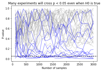
In this picture, each simulation run is a path which runs from zero samples to the total sample size. Paths which cross the $\alpha = .05$ line at any time would have been false positives under early stopping, and are colored blue. Paths which are never significant are shown in grey. You’ll notice that while few paths end below the dotted line, many of them cross the line of significance at some point as they bob up and down.

During these simulations, the T-test conducted at the very end had a false positive rate of 5%, as expected. But the procedure which allowed stopping every day (ie, every 100 samples) had a false positive rate of 27%, more than 5x worse! (I ran 1000 simulations, though I’m only showing 40 of them so the graph isn’t so busy - you can find the code in the appendix, if you’re curious.)

We talked about the speed-risk tradeoff before - adding more checks without changing anything else will expose us to more risks, and make our test results much less safe. How should we insulate ourselves from the risk of a false positive if we want to stop early?

On first glance, this looks similar to the problem of multiple testing that might be addressed by methods like the Bonferroni correction or an FDR correcting method. Those methods also help us out in situations where more checks inflate the false positive rate. Those methods would cause us to set our $\alpha$ lower based on the number of checks we’re planning to run. By lowering $\alpha$ we are “raising the bar” and demanding more evidence before we accept a result. This is a good start, but it has a serious flaw - it will meaningfully decrease the power ($\beta$) of our experiment, and we’ll need to run it longer than expected. Can we do better?

We can try and compromise by saying that we should be skeptical of apparent effects early in the experiment, but that effects that are really large should still prompt us to stop early. That leaves us a little wiggle room - we should not stop early most of the time, unless the effect looks like it is really strong. What if we set $\alpha$ lower at the beginning of the experiment, but used the original value of $\alpha$ (5%, or whatever) after all the data is collected? That sort of “early skepticism” approach might get us a procedure that works.

Of course, the devil is in the details, and so this opens us up to the next question. How strong does the effect need to be early on in the experiment for us to be willing to stop early? How should we change our testing procedure to accommodate early stopping?

The $\alpha$ spending function approach: set the standard evidence higher early on in the experiment

The idea we’ve come across here is called the alpha spending function approach. It works by turning our fixed significance level $\alpha$ into a function $adjust(p, \alpha)$, which takes in the proportion of the sample we’ve collected so far and tells us how to adjust the significance level based on how far along we are. The proportion $p$ is given by $p = \frac{n}{N}$, the fraction of the total sample collected.

The idea here is that when $p$ is small, $\alpha$ will be small, and we’ll be very skeptical of observed effects. When we’ve collected the entire sample then $p = 1$ and we’ll apply no adjustment, meaning $adjust(p, \alpha) = \alpha$. A detailed reference here is Lan and DeMets 1994, which focuses on the clinical trial setting.

What form might $adjust(p, \alpha)$ have? Since we want it to scale between 0 and $\alpha$ as $p$ increases, a reasonable starting point is something like:

We might called this a linear alpha spending function. Lan and Demets above mention an alternative called the O’Brien-Fleming (OBF) alpha spending function, which is:

Where $\Phi$ is the CDF of a standard normal distribution, $Z_{\alpha/2}$ is the Z-value associated with $\alpha/2$, and $p$ is the fraction of the sample we’ve collected so far.

In Python, a little bit of assembly is required to calculate this function. It looks something like this:

def obf_alpha_spending(desired_final_alpha, proportion_sample_collected):
    z_alpha_over_2 = norm.ppf(1-desired_final_alpha/2)
    return 2 - 2*(norm.cdf(z_alpha_over_2/np.sqrt(proportion_sample_collected)))

Unless you spend a lot of time thinking about the normal CDF, it’s probably not obvious what this function looks like. Lets see how going from $p=0$ (none of the sample collected) to $p=1$ (full sample collected) looks:

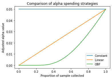
We see that the OBF function is more conservative everywhere than the linear function, but that it is extra conservative at the beginning. Why might this be? Some intuition (I think) has to do with the fact that the relationship between sample size and precision is non-linear (the formula for the standard error of the mean, for example, includes a $\sqrt{n}$).

Okay, so we have a way of adjusting $\alpha$ dependign on how much data has arrived. Lets put it to the test. We’ll rerun the simulation above, with the following conditions. This time, we’ll compare the false positive rates from the different strategies we’ve discussed: constant alpha (same as above), the linear spending function, and the O’Brien Fleming spending function. The results of 10,000 simulated experiments look like this:

In the first row, we see what we already know - early stopping without using an alpha spending rule has a False positive rate much larger than the expected 5%. Linear alpha spending is an improvement (about 2.6x more errors than desired), but OBF is the winner, with a Type I error rate closest to 5% (1.6x more errors than desired). OBF will have less power, but power analysis subject to early stopping rules is a subject for another time.

The alpha spending approach is an easy thing to add to your next test, and it’s worth doing - it lets you have the best of both worlds, letting you stop early if the result is large at only a small cost to your false positive rate. And given that you can write it as a 2-line Python function, it’s not too hard to add to your A/B test analysis tool. And best of all, having a strategy for early stopping means no more awkward conversations about the arcane mystic powers of ✨S T A T I S T I C S✨ with your cross-functional partners!

Appendix: Code for the simulations

P-value paths

import numpy as np
from scipy.stats import ttest_ind, norm
import pandas as pd

days_in_test = 30
samples_per_day = 100


def simulate_one_experiment():
    treated_samples, control_samples = np.array([]), np.array([])
    
    simulation_results = []
    
    for day in range(days_in_test):
        treated_samples = np.append(treated_samples, np.random.exponential(5, size=samples_per_day))
        control_samples = np.append(control_samples, np.random.normal(5, size=samples_per_day))
        result = ttest_ind(treated_samples, control_samples)
        simulation_results.append([day, len(treated_samples), result.statistic, result.pvalue])
        
    simulation_results = pd.DataFrame(simulation_results, columns=['day', 'n', 't', 'p'])
    return simulation_results

from matplotlib import pyplot as plt
import seaborn as sns

n_simulations = 40
false_positives = 0
early_stop_false_positives = 0

for i in range(n_simulations):
    result = simulate_one_experiment()
    if np.any(result['p'] <= .05):
        early_stop_false_positives += 1
        color = 'blue'
        alpha = 0.5
    else:
        color = 'grey'
        alpha = .3
    if result.iloc[-1]['p'] <= .05:
        false_positives += 1
    plt.plot(result['n'], result['p'], color=color, alpha=alpha)

plt.axhline(.05, linestyle='dashed', color='black')
plt.xlabel('Number of samples')
plt.ylabel('P-value')
plt.title('Many experiments will cross p < 0.05 even when H0 is true')
print('False positives with full sample:', false_positives / n_simulations)
print('False positives if early stopping is allowed:', early_stop_false_positives / n_simulations)

Plotting the OBF function

from scipy.stats import norm
import numpy as np
from matplotlib import pyplot as plt

def constant_alpha(desired_final_alpha, proportion_sample_collected):
    return desired_final_alpha

def linear_alpha_spending(desired_final_alpha, proportion_sample_collected):
    return proportion_sample_collected * desired_final_alpha

def obf_alpha_spending(desired_final_alpha, proportion_sample_collected):
    z_alpha_over_2 = norm.ppf(1-desired_final_alpha/2)
    return 2 - 2*(norm.cdf(z_alpha_over_2/np.sqrt(proportion_sample_collected)))

p = np.linspace(0, 1, 100)
alpha = .05
plt.plot(p, [constant_alpha(alpha, pi) for pi in p], label='Constant')
plt.plot(p, [linear_alpha_spending(alpha, pi) for pi in p], label='Linear')
plt.plot(p, [obf_alpha_spending(alpha, pi) for pi in p], label='OBF')
plt.legend()
plt.xlabel('Proportion of sample collected')
plt.ylabel('Adjusted alpha value')
plt.title('Comparison of alpha spending strategies')

Type I error comparison of different alpha spending functions

import pandas as pd
import numpy as np
from scipy.stats import ttest_ind, norm
from tqdm import tqdm

def constant_alpha(desired_final_alpha, proportion_sample_collected):
    return desired_final_alpha

def linear_alpha_spending(desired_final_alpha, proportion_sample_collected):
    return proportion_sample_collected * desired_final_alpha

def obf_alpha_spending(desired_final_alpha, proportion_sample_collected):
    z_alpha_over_2 = norm.ppf(1-desired_final_alpha/2)
    return 2 - 2*(norm.cdf(z_alpha_over_2/np.sqrt(proportion_sample_collected)))

def simulate_one(control_average, alpha_strategies, samples_per_day, number_of_days, desired_final_alpha):
    total_sample_size = samples_per_day * number_of_days
    results = {f.__name__: 0 for f in alpha_strategies}
    control_samples, treatment_samples = np.array([]), np.array([])
    for day in range(number_of_days):
        control_samples = np.concatenate([control_samples, np.random.exponential(scale=control_average, size=samples_per_day)])
        treatment_samples = np.concatenate([treatment_samples, np.random.exponential(scale=control_average, size=samples_per_day)])
        for alpha_strategy in alpha_strategies:
            alpha = alpha_strategy(desired_final_alpha, len(control_samples) / total_sample_size)
            if ttest_ind(control_samples, treatment_samples).pvalue <= alpha:
                results[alpha_strategy.__name__] = 1
    return results

simulation_results = pd.DataFrame([simulate_one(control_average=5, 
                                                alpha_strategies=[constant_alpha, linear_alpha_spending, obf_alpha_spending], 
                                                samples_per_day=100, 
                                                number_of_days=30, 
                                                desired_final_alpha=.05) for _ in tqdm(range(10000))])

print(simulation_results.mean())
print(simulation_results.sum())

Pipelines make model specification easy

Most of the time, ML models can’t just suck in data from the world and spit predictions back out, whaterver overzealous marketers of the latest AI fad might tell you. Usually, you need a bit of careful sculpting of the input matrix in order to make sure it is usable by your favorite model. For example, you might do things like:

• Scale variables by setting them from 0 to 1 or normalizing them
• Encoding non-numeric values as one-hot vectors
• Generating spline features for continues numeric values
• Running some function on the inputs values, like sqrt(x)

In Python, this process is eased quite a bit by the usage of Scikit-learn Pipelines, which let you chain together as many preprocessing steps as you like and then treat them like one big model. The idea here is that stateful transformations are basically part of your model, so you should fit/transform them the same way you do your model. The FunctionTransformer allows you to perform stateless transformations. In order to create a stateful transformations, you’ll need to write your own Transformer class - but luckily, it’s pretty easy once you have an idea of how to structure it.

Anatomy of an Sklearn Transformer

Creating a subclass is as easy as inheriting from BaseEstimator and TransformerMixin and writing a couple of methods which might be familiar if you’ve been using scikit-learn already:

• fit(X, y): This method takes care of any state you need to track. In the scaling example, this means computing the observed min and max of each feature, so we can scale inputs later.
• transform(X): This method applies the change. In the scaling example, this means subtracting the min value and dividing by the max, both of which were stored previously.

For example, if you wanted to write a transformer that centered data by subtracting its mean (de-meaning it? that feels too mean), its fit and transform would do the following:

• fit(X, y): Calculate the average of each column (ie, take the vector average of X).
• transform(X): Subtract the stored average from the input vectors in X.

Lets take a look at a couple of examples that I’ve found useful in my work.

An example: Replace a rare token in a column with some value

A common trick in dealing with categorical columns in ML models is to replace rare categories with a unique value that indicates “Other” or “This is a rare value”. This kind of prepreocessing would be handy to have available as a transformer, so let’s build one.

At init time, we’ll take in parameters from the user:

• target_column - The column to scan
• min_pct - Values which appear in a smaller percentage of rows than this will be considered rare
• min_count - Values which appear in fewer rows than this will be considered rare. Mutually exclusive with the previous
• replacement_token - The token to convert rare values to.

We can sketch out the fit and transform methods:

• fit(X, y): Look at examples of target_column and find examples of tokens with less than min_pct or min_count. Store them in the object’s state.
• transform(X): Look at the target_column, and replace all the known rare tokens with the replacement token.

Here’s what that looks like in code as a transformer subclass:

class RareTokenTransformer(BaseEstimator, TransformerMixin):
    def __init__(self, target_column, min_pct=None, min_count=None, replacement_token='__RARE__'):
        self.target_column = target_column
        if (min_pct and min_count) or (not min_pct and not min_count):
            raise Exception("Please provide either min_pct or min_count, not both")
        self.min_pct = min_pct
        self.min_count = min_count
        self.replacement_token = replacement_token
    
    def fit(self, X, y=None):
        counts = X[self.target_column].value_counts()
        if self.min_count:
            rare_tokens = set(counts.index[counts <= self.min_count])
        if self.min_pct:
            pcts = X[self.target_column].value_counts() / counts.sum()
            rare_tokens = set(pcts.index[pcts <= self.min_pct])
        self.rare_tokens = rare_tokens
        return self
    
    def transform(self, X):
        X_copy = X.copy()
        X_copy[self.target_column] = X_copy[self.target_column].replace(self.rare_tokens, self.replacement_token)
        return X_copy

Let’s try it on a real dataframe.

X1 = pd.DataFrame({'numeric_col': [0, 1, 2, 3, 4], 'categorical_col': ['A', 'A', 'A', 'B', 'C']})
X2 = pd.DataFrame({'numeric_col': [0, 1, 2, 3, 4], 'categorical_col': ['C', 'A', 'B', 'A', 'A']})

t = RareTokenTransformer('categorical_col', min_pct=0.2)
t.fit(X1)
print(t.transform(X1).to_markdown())
print(t.transform(X2).to_markdown())

This gives us the expected X1:

And X2:

A borrowed example: Combining patsy and sklearn

One of the few flaws of Scikit-learn is that it doesn’t include out-of-the-box support for Patsy. Patsy is a library that lets you easily specify design matrices with a single string. Statsmodels allows you to fit models specified using Patsy strings, but Statsmodels only really covers generalized linear models.

It would be really handy to be able to use scikit-learn models with Patsy. A FormulaTransformer is implemented by Dr. Juan Camilo Orduz on his blog that does just that - I’ve borrowed his idea here and modified it to make it stateful.

This transformer will include the following fit and transform steps:

• fit(X, y): Compute the design_info based on the specified formula and X. For example, Patsy needs to keep track of which columns are categorical and which are numeric.
• transform(X): Run patsy.dmatrix using the design_info to generate the transformed version of X.

import patsy
from sklearn.base import BaseEstimator, TransformerMixin

class FormulaTransformer(BaseEstimator, TransformerMixin):
    # Adapted from https://juanitorduz.github.io/formula_transformer/
    def __init__(self, formula):
        self.formula = formula
    
    def fit(self, X, y=None):
        dm = patsy.dmatrix(self.formula, X)
        self.design_info = dm.design_info
        return self
    
    def transform(self, X):
        X_formula = patsy.dmatrix(formula_like=self.formula, data=X)
        columns = X_formula.design_info.column_names
        X_formula = patsy.build_design_matrices([self.design_info], X, return_type='dataframe')[0]
        return X_formula

Lets take a look at how this transforms an actual dataframe. We’ll use input matrices with one numeric and one categorical column. We’ll square the numeric column, and one-hot encode the categorical one.

import pandas as pd
import numpy as np
pd.set_option('display.max_columns', None)

X1 = pd.DataFrame({'numeric_col': [0, 1, 2], 'categorical_col': ['A', 'B', 'C']})
X2 = pd.DataFrame({'numeric_col': [0, 1, 2], 'categorical_col': ['C', 'A', 'B']})

t = FormulaTransformer('np.power(numeric_col, 2) + categorical_col - 1')
t.fit(X1)
print(t.transform(X1).to_markdown())
print(t.transform(X2).to_markdown())

This shows us what we expect, namely that X1 is:

And that X2 is:

It’s everywhere!

I have spent a shocking percentage of my career drawing some version of this diagram on a whiteboard:

This relationship has a few key aspects that I notice over and over again:

• The output increases when more input is added; the line slopes up.
• Each input added is less efficient than the last; the slope is decreasing.
• Inputs and outputs are both positive

There’s also a downward-sloping variant, and a lot of the same analysis goes into that as well.

If you’re an economist, or even if you just took econ 101, you likely recognize this. It’s common to model this kind of relationship as $y = ax^b$, a function which has “constant elasticity”, meaning an percent change in input produces the same percent change in output regardless of where you are in the input space. A common example is the Cobb-Douglas production function. The most common examples all seem to be related to price, such as how changes in price affect the amount demanded or supplied.

Lots and lots and lots of measured variables seem to have this relationship. In my own career I’ve seen this shape of input-output relationship show up over and over, even outside the price examples:

• Marketing spend and impressions
• Number of users who see something vs the number who engage with it
• Number of samples vs model quality
• Time spent on a project and quality of result
• Size of an investment vs revenue generated (this one was popularized and explored by a well known early data scientist)

To get some intuition, lets look at some examples of how different values of $\alpha$ and $\beta$ affect the shape of this function:

x = np.linspace(.1, 3)

def f(x, a, b):
  return a*x**b

plt.title('Examples of ax^b')
plt.plot(x, f(x, 1, 0.5), label='a=1,b=0.5')
plt.plot(x, f(x, 1, 1.5), label='a=1,b=1.5')
plt.plot(x, f(x, 1, 1.0), label='a=1,b=1.0')
plt.plot(x, f(x, 3, 0.5), label='a=2,b=0.5')
plt.plot(x, f(x, 3, 1.5), label='a=2,b=1.5')
plt.plot(x, f(x, 3, 1.0), label='a=2,b=1.0')
plt.legend()
plt.show()

By and large, we see that $\alpha$ and $\beta$ are the analogues of the intercept and slope, that is

• $\alpha$ affects the vertical scale, or where the curve is anchored when $x=0$
• $\beta$ affects the curvature (when $\beta < 1$, there are diminishing returns; when $\beta > 1$ increasing returns, when $\beta = 0$ then it’s linear). When it’s negative, the slope is downward.

Nonetheless, I am not an economist (though I’ve had the pleasure of working with plenty of brilliant people with economics training). If you’re like me, then you might not have these details close to hand. This post is meant to be a small primer for anyone who needs to build models with these kinds of functions.

We usually want to know this relationship so we can answer some practical questions such as:

• How much input will we need to add in order to reach our desired level of output?
• If we have some free capital, material, or time to spend, what will we get for it? Should we use it here or somewhere else?
• When will it become inefficient to add more input, ie when will the value of the marginal input be less than the marginal output?

Let’s look at the $ \alpha x ^\beta$ model in detail.

Some useful facts about the $y = \alpha x ^\beta$ model

It makes it easy to talk about % change in input vs % change in output

One of the many reasons that the common OLS model $y = \alpha + \beta x$ is so popular is that it lets us make a very succinct statement about the relationship between $x$ and $y$: “A one-unit increase in $x$ is associated with an increase of $\beta$ units of $y$.” What’s the equivalent to this for our model $y = \alpha x ^ \beta$?

The interpretation of this model is a little different than the usual OLS model. Instead, we’ll ask: how does multiplying the input multiply the output? That is, how do percent changes in $x$ produce percent changes in $y$? For example, we might wonder what happens when we increase the input by 10%, ie multiplying it by 1.1. Lets see how multiplying the input by $m$ creates a multiplier on the output:

$\frac{f(xm)}{f(x)} = \frac{\alpha (xm)^\beta}{\alpha x ^ \beta} = m^\beta$

That means for this model, we can summarize changes between variables as:

Under this model, multiplying the input by m multiplies the output by $m^\beta$.

Or, if you are percentage afficionado:

Under this model, changing the input by $p\%$ changes the output output by $(1+p\%)^\beta$.

It’s easy to fit with OLS

Another reason that the OLS model is so popular is because it is easy to estimate in practice. The OLS model may not always be true, but it is often easy to estimate it, and it might tell us something interesting even if it isn’t correct. Some basic algebra lets us turn our model into one we can fit with OLS. Starting with our model:

$y = \alpha x^\beta$

Taking the logarithm of both sides:

$log \ y = log \ \alpha + \beta \ log \ x$

This model is linear in $log \ x$, so we can now use OLS to calculate the coefficients! Just don’t forget to $exp$ the intercept to get $\alpha$ on the right scale.

We can use it to solve for input if we know the desired level of output

In practical settings, we often start with the desired quantity of output, and then try to understand if the required input is available or feasible. It’s handy to have a closed form which inverts our model:

$f^{-1}(y) = (y/\alpha)^{\frac{1}{\beta}}$

If we want to know how a change in the output will require change in the input, we look at how multiplying the output by $m$ changes the required value of $x$:

$\frac{f^{-1}(ym)}{f^{-1}(y)} = m^{\frac{1}{\beta}}$

That means if our goal is to multiply the output by $m$ we need to multiply the input by $m^{\frac{1}{\beta}}$.

An example: Lotsize vs house price

Let’s look at how this relationship might be estimated on a real data set. Here, we’ll use a data set of house prices along with the size of the lot they sit on. The question of how lot size relates to house price has a bunch of the features we expect, namely:

• The slope is positive - all other things equal, we’d expect bigger lots to sell for more.
• Each input added is less efficient than the last; adding more to an already large lot probably doesn’t change the price much.
• Lot-size and price are both positive.

Lets grab the data:

from matplotlib import pyplot as plt
import seaborn as sns
import numpy as np
import pandas as pd 
from statsmodels.api import formula as smf

df = pd.read_csv('https://vincentarelbundock.github.io/Rdatasets/csv/AER/HousePrices.csv')
df = df.sort_values('lotsize')

We’ll fit our log-log model and plot it:

model = smf.ols('np.log(price) ~ np.log(lotsize)', df).fit()

plt.scatter(df['lotsize'], df['price'])
plt.plot(df['lotsize'], np.exp(model.fittedvalues), color='orange', label='Log-log model')
plt.title('Lot Size vs House Price')
plt.xlabel('Lot Size')
plt.ylabel('House Price')
plt.legend()
plt.tight_layout()
plt.show()

Okay, looks good so far. This seems like a plausible model for this case. Let’s double check it by looking at it on the log scale:

plt.scatter(df['lotsize'], df['price'])
plt.plot(df['lotsize'], np.exp(model.fittedvalues), label='Log-log model', color='orange')
plt.xscale('log')
plt.yscale('log')
plt.title('LogLot Size vs Log House Price')
plt.xlabel('Log Lot Size')
plt.ylabel('Log House Price')
plt.legend()
plt.tight_layout()
plt.show()

Nice. When we log-ify everything, it looks like a textbook regression example.

Okay, let’s interpret this model. Lets convert the point estimate of $\beta$ into an estimate of percent change:

b = model.params['np.log(lotsize)']
a = np.exp(model.params['Intercept'])
print('1% increase in lotsize -->', round(100*(1.01**b-1), 2), '% increase in price')
print('2% increase in lotsize -->', round(100*(1.02**b-1), 2), '% increase in price')
print('10% increase in lotsize -->', round(100*(1.10**b-1), 2), '% increase in price')

1% increase in lotsize --> 0.54 % increase in price
2% increase in lotsize --> 1.08 % increase in price
10% increase in lotsize --> 5.3 % increase in price

We see that relatively, price increases more slowly than lotsize.

Does this model really describe reality? A reminder that a convenient model need not be the correct model

The above set of tips and tricks is, when you get down to it, mostly algebra. It’s useful algebra to be sure, but it is really just repeated manipulation of the functional form $\alpha x ^ \beta$. It turns out that that functional form is both a priori plausible for lots of relationships, and is easy to work with.

However, we should not mistake analytical convenience for truth. We should recognize that assuming a particular functional form comes with risks, so we should spend some time:

• Demonstrating that this functional form is a good fit for the data at hand by doing regression diagnostics like residual plots
• Understanding how far off our model’s predictions and prediction intervals are from the truth by doing cross-validation
• Making sure we’re clear on what causal assumptions we’re making, if we’re going to consider counterfactuals

This is always good practice, of course - but it’s easy to forget about it once you have a particular model that is convenient to work with.

Some alternatives to the model we’ve been using

As I mentioned above, the log-log model isn’t the only game in town.

For one, we’ve assumed that the “true” function should have constant elasticity. But that need not be true; we could imagine taking some other function and computing its point elasticity in one spot, or its arc elasticity between two points.

What about alternatives to $y = \alpha x^\beta$ and the log-log model?

• If you just want a model that is non-decreasing or non-increasing, you could try non-parametric isotonic regression.
• You could pick a different transformation other than log, like a square root. This also works when there are zeros, whereas $log(0)$ is undefined.
• Another possible transformation is Inverse Hyperbolic Sine, which also has an elasticity interpreation.

Appendix: Estimating when you have only two data points

Occasionally I’ve gone and computed an observed elasticity by fitting the model from a single pair of observations. This isn’t often all that useful, but I’ve included it here in case you find it helpful.

Lets imagine we have only two data points, which we’ll call $x_1, y_1, x_2, y_2$. Then, we have two equations and two unknowns, that is:

If we do some algebra, we can come up with estimates for each variable:

import numpy as np
def solve(x1, x2, y1, y2):
    # y1 = a*x1**b
    # y2 = a*x2**b
    log_x1, log_x2, log_y1, log_y2 = np.log(x1), np.log(x2), np.log(y1), np.log(y2)
    b = (log_y1 - log_y2) / (log_x1 - log_x2)
    log_a = log_y1 + b*log_x1
    return np.exp(log_a), b

Then, we can run an example like this one in which a 1% increase in $x$ leads to a 50% increase in $y$:

a, b = solve(1, 1.01, 1, 1.5)
print(a, b, 1.01**b)

Which shows us a=1.0, b=40.74890715609402, 1.01^b=1.5.

This doesn’t usually answer our question, though. Model selection tells us which choice is the best among the available options, but it’s unclear whether even the best one is actually good enough to be useful. I myself have had the frustrating experience of performing an in-depth model selection process, only to realize at the end that all my careful optimizing has given me a model which is better than the baseline, but still so bad at predicting that it is unusable for any practical purpose.

So, back to our question. What does “accurate enough to be useful” mean, exactly? How do we know if we’re there?

We could try imposing a rule of thumb like “your MSE must be this small”, but this seems to require context. After all, different tasks require different levels of precision in the real world - this is why dentists do not (except in extreme situations) use jackhammers, preferring tools with a diameter measured in millimeters.

Statistical measures of model or coefficient significance don’t seem to help either; knowing that a given coefficient (or all of them) are statistically significantly different from zero is handy, but does not tell us that the model is ready for prime time. Even the legendary $R^2$ doesn’t really have a clear a priori “threshold of good enough” (though surprisingly, I see to frequently run into people who are willing to do so, often claiming 80% or 90% as if their model is trying to make the Honor Roll this semester). If you’re used to using $R^2$, a perspective I found really helpful is Ch. 10 of Cosma Shalizi’s The Truth About Linear Regression.

An actual viable method is to look at whether your prediction intervals are both practically precise enough for the task and also cover the data, an approach detailed here. This is a perfectly sensible choice if your model provides you with an easy way to compute prediction intervals. However, if you’re using something like scikit-learn you’ll usually be creating just a single point estimate (ie, a single fitted model of $\mathbb{E}[y \mid X]$ which you can deploy), and it may not be easy to generate prediction intervals for your model.

The method that I’ve found most effective is to work with my stakeholders and try to determine what size of relative (percent) error would be good enough for decision making, and then see how often the model predictions meet that requirement. Usually, I ask a series of questions like:

• Imagine the model was totally accurate and precise, ie it hit the real value 100% of the time. What would that let us do? What value would that success bring us in terms of outcomes? Presumably, there is a clear answer here, and this would let us increase output, sell more products, or something else we want.
• Now imagine that the model’s accuracy was off by a little bit, say 5%. Would you still be able to achieve the desired outcome?
• If so, what if it was 10%? 20%? How large could the error be and still allow you to achieve your desired outcome?
• Take this threshold, and consider every prediction within it to be a “hit”, and everything else is a “miss”. In that case, we can evaluate the model’s practical usefulness by seeing how often it produces a hit.

This allows us to take our error measure, which is a continuous number, and discretize it. We could add more categories by defining what it means to have a “direct hit”, a “near miss”, a “bad miss” etc. You could then attach a predicted outcome to each of those discrete categories, and you’ve learned something not just about how the model makes predictions, but how it lets you make decisions. In this sense, it’s the regression-oriented sequel to our previous discussion about analyzing the confusion matrix for classifiers - we go from pure regression analysis to decision analysis using a diagnostic. The “direct hits” for a regression model are like landing in the main diagonal of the confusion matrix.

In a sense, this is a check of the model’s “calibration quality”. While I usually hear that term referring to probability calibration, I think it’s relevant here too. In the regression setting, a model is “well calibrated” when its prediction are at or near the actual value. We’ll plot the regression equivalent of the calibration curve, and highlight the region that counts as a good enough fit.

Let’s do a quick example using this dataset of California House Prices along with their attributes. Imagine that you’re planning on using this to figure out what the potential price of your house might be when you sell it; you want to know how much you might get for it so you can figure out how to budget for your other purchases. We’ll use a Gradient Boosting model, but that’s not especially important - whatever black-box method you’re using should work.

First, lets get all our favorite toys out of the closet, grabbing our data and desired model:

import pandas as pd
import numpy as np
from sklearn.model_selection import cross_val_predict
from sklearn.ensemble import HistGradientBoostingRegressor
from sklearn.datasets import fetch_california_housing

california_housing = fetch_california_housing(as_frame=True)
data = california_housing.frame

input_features = ['MedInc', 'HouseAge', 'AveRooms', 'AveBedrms', 'Population', 'AveOccup', 'Latitude', 'Longitude']
target_variable = 'MedHouseVal'

X = data[input_features]
y = data[target_variable]

model = HistGradientBoostingRegressor()

In this context, the acceptable amount of error is probably dictated by how much money you have in the bank as a backup in case you get less for the house than you expected. For your purposes, you decide that a difference of 35% compared to the actual value would be too much additional cost for you to bear.

We’ll first come up with out-of-sample predictions using the cross validation function, and then we’ll plot the actual vs predicted values along with the “good enough” region we want to hit.

predictions = cross_val_predict(model, X, y, cv=5)  # cv=5 for 5-fold cross-validation

from matplotlib import pyplot as plt
import seaborn as sns

x_y_line = np.array([min(predictions), max(predictions)])
p = 0.35 # Size of threshold, 35%

sns.histplot(x=predictions, y=y) # Plot the predicted vs actual values
plt.plot(x_y_line, x_y_line, label='Perfect accuracy', color='orange') # Plot the "perfect calibration" line
plt.fill_between(x_y_line, x_y_line*(1+p), x_y_line*(1-p), label='Acceptable error region', color='orange', alpha=.1) # Plot the "good enough" region
plt.xlabel('Predicted')
plt.ylabel('Actual')
plt.legend()
plt.show()

For reasons I can’t really explain, I find it very amusing that this diagram looks like the flag of Seychelles, and would look even more so if we added finer gradations of hit vs missed targets.

In addition to a chart like this, it’s also handy to define a numeric score - we could even use this for model selection, if we wanted to. One that seems like it would be an easy step to me is the percentage of time our model makes predictions that land in the bound of acceptable error. Hopefully, that number is high, indicating that we can usually expect this model to produce outputs of good enough quality to use for decision-making.

If we define $p$ as the acceptable percent change, we can compute the estimated percent of predictions within acceptable error as:

To think about this from an engineering perspective, our use case defines the “tolerance”, similar to the tolerance which is set in machining parts. This quantity tells us how often the product which our model produces (ie its output) is within the tolerance for error that we can handle.

# Within target region calculation

within_triangle = sum((y*(1-p) < predictions) & (predictions < y*(1+p)))

print(round(100 * (within_triangle / len(y))), 2)

That gives us 66% for this model on this data set - a strong start, though there’s probably room for improvement. It seems unlikely that we’d be willing to deploy this model as-is, and we’d want to improve performance by adding more features, more data, or improving the model design. However, even though this model is not usable currently, it’s useful to now have a way of measuring how well the model fits the task at hand.

This is just one example of doing decision-oriented model validation, but the method could be expanded or taken in different directions. If we wanted to get a finer idea of how our decisions might play out, we could break the plot into more segments, like introducing regions for “near misses” or “catastrophic misses”. You could also probably analyze the relationship between predicted and actual with quantile regression, learning what the “usual” lower bound on actual value given the predicted value is.

It’s generally good to try and guess what the future will look like, so we can plan accordingly. How much will our new inventory cost? How many users will show up tomorrow? How much raw material will I need to buy? The first instinct we have is usual to look at historical averages; we know the average price of widgets, the average number of users, etc. If we’re feeling extra fancy, we might build a model, like a linear regression, but this is also an average; a conditional average based on some covariates. Most out-of-the-box machine learning models are the same, giving us a prediction that is correct on average.

However, answering these questions with a single number, like an average, is a little dangerous. The actual cost will usually not be exactly the average; it will be somewhat higher or lower. How much higher? How much lower? If we could answer this question with a range of values, we could prepare appropriately for the worst and best case scenarios. It’s good to know our resource requirements for the average case; it’s better to also know the worst case (even if we don’t expect the worst to actually happen, if total catastrophe is plausible it will change our plans).

As is so often the case, it’s useful to consider a specific example. Let’s imagine a seasonal product; to pick one totally at random, imagine the inventory planning of a luxury sunglasses brand for cats. Purrberry needs to make summer sales projections for inventory allocation across its various brick-and-mortar locations where it’s sales happen.

You go to your data warehouse, and pull last year’s data on each location’s pre-summer sales (X-axis) and summer sales (Y-axis):

from matplotlib import pyplot as plt
import seaborn as sns

plt.scatter(df['off_season_revenue'], df['on_season_revenue'])
plt.xlabel('Off season revenue at location')
plt.ylabel('On season revenue at location')
plt.title('Comparison between on and off season revenue at store locations')
plt.show()

We can read off a few things here straight away:

• A location with high off-season sales will also have high summer sales; X and Y are positively correlated.
• The outcomes are more uncertain for the stores with the highest off-season sales; the variance of Y increases with X.
• On the high end, outlier results are more likely to be extra high sales numbers instead of extra low; the noise is asymmetric, and positively skewed.

After this first peek at the data, you might reach for that old standby, Linear Regression.

Our usual tool, OLS, doesn’t always handle this well

Regression afficionados will recall that our trusty OLS model allows us to compute prediction intervals, so we’ll try that first.

Recall that the OLS model is

$y ~ \alpha + \beta x + N(0, \sigma)$

Where $\alpha$ is the intercept, $\beta$ is the slope, and $\sigma$ is the standard deviation of the residual distribution. Under this model, we expect that observations of $y$ are normally distributed around $\alpha + \beta x$, with a standard deviation of $\sigma$. We estimate $\alpha$ and $\beta$ the usual way, and look at the observed residual variance to estimate $\sigma$, and we can use the familiar properties of the normal distribution to create prediction intervals.

from statsmodels.api import formula as smf

ols_model = smf.ols('on_season_revenue ~ off_season_revenue', df).fit()
predictions = ols_model.predict(df)
resid_sd = np.std(ols_model.resid)

high, low = predictions + 1.645 * resid_sd, predictions - 1.645 * resid_sd

plt.scatter(df['off_season_revenue'], df['on_season_revenue'])
plt.plot(df['off_season_revenue'], high, label='OLS 90% high PI')
plt.plot(df['off_season_revenue'], predictions, label='OLS prediction')
plt.plot(df['off_season_revenue'], low, label='OLS 90% low PI')
plt.legend()
plt.xlabel('Off season revenue at location')
plt.ylabel('On season revenue at location')
plt.title('OLS prediction intervals')
plt.show()

Hm. Well, this isn’t terrible - it looks like the 90% prediction intervals do contain the majority of observations. However, it also looks pretty suspect; on the left side of the plot the PIs seem too broad, and on the right side they seem a little too narrow.

This is because the PIs are the same width everywhere, since we assumed that the variance of the residuals is the same everywhere. But from this plot, we can see that’s not true; the variance increases as we increase X. These two situations (constant vs non-constant variance) have the totally outrageous names homoskedasticity and heteroskedasticity. OLS assumes homoskedasticity, but we actually have heteroskedasticity. If we want to make predictions that match the data we see, and OLS model won’t quite cut it.

NB: A choice sometimes recommended in a situation like this is to perform a log transformation, but we’ve seen before that logarithms aren’t a panacea when it comes to heteroskedasticity, so we’ll skip that one.

The idea: create prediction intervals based on the conditional quantiles

We really want to answer a question like: “For all stores with $x$ in pre-summer sales, where will (say) 90% of the summer sales per store be?”. We want to know how the bounds of the distribution, the highest and lowest plausible observations, change with the pre-summer sales numbers. If we weren’t considering an input like the off-season sales, we might look at the 5% and 95% quantiles of the data to answer that question.

We want to know what the quantiles of the distribution will be if we condition on $x$, so our model will produce the conditional quantiles given the off-season sales. This is analogous to the conditional mean, which is what OLS (and many machine learning models) give us. The conditional mean is $\mathbb{E}[y \mid x]$, or the expected value of $y$ given $x$. We’ll represent the conditional median, or conditional 50th quantile, as $Q_{50}[y \mid x]$. Similarly, we’ll call the conditional 5th percentile $Q_{5}[y \mid x]$, and the conditional 95th percentile will be $Q_{95}[y \mid x]$.

OLS works by finding the coefficients that minimize the sum of the squared loss function. Quantile regression can be framed in a similar way, where the loss function is changed to something else. For the median model, the minimization happening is LAD, a relative of OLS. For a model which computes arbitrary quantiles, we mininimize the whimsically named pinball loss function. You can look at this section of the Wikipedia page to learn about the minimization problem happening under the hood.

Quantile regression in action

Fitting the model

As usual, we’ll let our favorite Python library do the hard work. We’ll build our quantile regression models using the statsmodels implementation. The interface is similar to the OLS model in statsmodels, or to the R linear model notation. We’ll fit three models: one for the 95th quantile, one for the median, and one for the 5th quantile.

high_model = smf.quantreg('on_season_revenue ~ off_season_revenue', df).fit(q=.95)
mid_model = smf.quantreg('on_season_revenue ~ off_season_revenue', df).fit(q=.5)
low_model = smf.quantreg('on_season_revenue ~ off_season_revenue', df).fit(q=.05)

plt.scatter(df['off_season_revenue'], df['on_season_revenue'])
plt.plot(df['off_season_revenue'], high_model.predict(df), label='95% Quantile')
plt.plot(df['off_season_revenue'], mid_model.predict(df), label='50% Quantile (Median)')
plt.plot(df['off_season_revenue'], low_model.predict(df), label='5% Quantile')
plt.legend()
plt.xlabel('Off season revenue at location')
plt.ylabel('On season revenue at location')
plt.title('Quantile Regression prediction intervals')
plt.show()

The 90% prediction intervals given by these models (the range between the green and blue lines) look like a much better fit than those given by the OLS model. On the left side of the X-axis, the interval is appropriately narrow, and then widens as the X-axis increases. This change in width indicates that our model is heteroskedastic.

It also looks like noise around the median is asymmetric; the distance from the upper bound to the median looks larger than the distance from the lower bound to the median. We could see this in the model directly by looking at the slopes of each line, and seeing that $\mid \beta_{95} - \beta_{50} \mid \geq \mid \beta_{50} - \beta_{5} \mid$.

Checking the model

Being careful consumers of models, we are sure to check the model’s performance to see if there are any surprises.

First, we can look at the prediction quality in-sample. We’ll compute the coverage of the model’s predictions. Coverage is the percentage of data points which fall into the predicted range. Our model was supposed to have 90% coverage - did it actually?

from scipy.stats import sem
covered = (df['on_season_revenue'] >= low_model.predict(df)) & (df['on_season_revenue'] <= high_model.predict(df))
print('In-sample coverage rate: ', np.average(covered))
print('Coverage SE: ', sem(covered))

In-sample coverage rate:  0.896
Coverage SE:  0.019345100974843932

The coverage is within one standard error of 90%. Nice!

There’s no need to limit ourselves to looking in-sample and we probably shouldn’t. We could use the coverage metric during cross-validation, ensuring that the out-of-sample coverage was similarly good.

When we do OLS regression, we often plot the predictor against the error to understand whether the linear specification was reasonable. We can do the same here by plotting our predictor against the coverage. This plot shows the coverage and a CI for each quartile.

sns.regplot(df['off_season_revenue'], covered, x_bins=4)
plt.axhline(.9, linestyle='dotted', color='black')
plt.title('Coverage by revenue group')
plt.xlabel('Off season revenue at location')
plt.ylabel('Coverage')
plt.show()

All the CIs contain 90% with no clear trend, so the linear specification seems reasonable. We could make the same plot by decile, or even percentile as well to get a more careful read.

What if that last plot had looked different? If the coverage veers off the the target value, we could have considered introducing nonlinearities to the model, such as adding splines.

Some other perspectives on quantile regression and prediction intervals

This is just one usage of quantile regression. QR models can also be used for multivariable analysis of distributional impact, providing very rich summaries of how our covariates are correlated with change in the shape of the output distribution.

We also could have thought about prediction intervals differently. If we believed that the noise was heteroskedastic but still symmetric (or perhaps even normally distributed), we could have used an OLS-based procedure model how the residual variance changed with the covariate. For a great summary of this, see section 10.3 of Shalizi’s data analysis book.

Appendix: How the data was generated

The feline fashion visionaries at Purrberry are, regrettably, entirely fictional for the time being. The data from this example was generated using the below code, which creates skew normal distributed noise:

import numpy as np
from scipy.stats import skewnorm
import pandas as pd

n = 250
x = np.linspace(.1, 1, n)
gen = skewnorm(np.arange(len(x))+.01, scale=x)
gen.random_state = np.random.Generator(np.random.PCG64(abs(hash('predictions'))))
y = 1 + x + gen.rvs()

df = pd.DataFrame({'off_season_revenue': x, 'on_season_revenue': y})

Distributional effects of A/B tests are often overlooked but provide a deeper understanding

The group averages and average treatment effect hide a lot of information

Most companies I know of that include A/B testing in their product development process usually do something like the following for most of their tests:

• Pick your favorite metric which you want to increase, and perhaps some other metrics that will act as guard rails. Often, this is some variant of “revenue per user”, “engagment per user”, ROI or the efficiency of the process.
• Design and launch an experiment which compares the existing product’s performance to that of some variant products.
• At some point, decide to stop collecting data.
• Compute the average treatment effect for the control version vs the test variant(s) on each metric. Calculate some measure of uncertainty (like a P-value or confidence/credible interval). Make a decision about whether to replace the existing production product with one of the test variants.

This process is so common because, well, it works - if followed, it will usually result in the introduction of product features which increase our favorite metric. It creates a series of discrete steps in the product space which attempt to optimize the favorite metric without incurring unacceptable losses on the other metrics.

In this process, the average treatment effect is the star of the show. But as we learn in Stats 101, two distributions can look drastically different while still having the same average. For example, here are four remarkably different distributions with the same average:

from matplotlib import pyplot as plt
import seaborn as sns
import numpy as np
from scipy.stats import poisson, skellam, nbinom, randint, geom

for dist in [poisson(100), skellam(1101, 1000), randint(0, 200), geom(1./100)]:
  plt.plot(np.arange(0, 400), dist.pmf(np.arange(0, 400)))
plt.xlim(0, 400)  
plt.ylabel('PMF')
plt.title('Four distributions with a mean of 100')
plt.show()

Similarly, the average treatment effect does not tell us much about how our treatment changed the shape of the distribution of outcomes. But we can expand our thinking not just to consider how the treatment changed the average, but the effect on the shape of the distribution; the distributional effect of the treatment. Expanding our thought to think about distributional effects might give us insights that we can’t get from averages alone, and help us see more clearly what our treatment did. For example:

• If we have a positive treatment effect, we can see whether one tail of the distribution was disproportionately affected. Did our gains come from lifting everyone? From squeezing more revenue out of the high-revenue users? From “lifting the floor” on the users who aren’t producing much in control?
• If an experiment negatively affected one tail of the distribution, we can consider mitigation. If our treatment provided a negative experience for users on the low end of the distribution, is there anything we can do to make their experience better?
• Are we meeting our goals for the shape of the distribution? For example, if we want to maintain a minimum service level, are we doing so in the treatment group?
• Do we want to move up market? If so, is our treatment increasing the output for the high end of the outcome distribution?
• Do we want to diversify our customer base? If so, is our treatment increasing our concentration among already high-value users?

The usual average treatment effect cannot answer these questions. We could compare single digit summaries of shape (variance, skewness, kurtosis) between treatment and control. However, even these are only simplified summaries; they describe a single attribute of the shape like the dispersion, symmetry, or heavy tailedness.

Instead, we’ll look at the empirical quantile function of control and treatment, and the difference between them. We’ll lay out some basic definitions here:

• The quantile function is the smooth version of the more familiar percentile distribution. For example, the 0.5 quantile is the median, the value that’s larger than 50% of the mass in the distribution, and the 50th percentile (those are all the same thing).
• The empirical quantile function is the set of quantile values in the treatment/control results which we actually observe.
• The inverse of the quantile function is the CDF , and its empirical counterpart is the empirical CDF. We won’t talk much about the CDF here, but it’s useful to link the two because the CDF is such a common description of a distribution.

Let’s take a look at an example of how we might use these in practice to learn about the distributional effects of a test.

An example: How did my A/B test affect the distribution of revenue?

Let’s once more put ourselves in the shoes of that most beloved of Capitalist Heroes, the purveyor of little tiny cat sunglasses. Having harnessed the illuminating insights of your business’ data, you’ve consistently been improving your key metric of Revenue per Cat. You currently send out a weekly email about the current purrmotional sales, a newsletter beloved by dashing calicos and tabbies the world over. As you are the sort of practical, industrious person who is willing to spend their valuable time reading a blog about statistics, you originally gave this email the very efficient subject line of “Weekly Newsletter” and move on to other things.

However, you’re realizing it’s time to revisit that decision - your previous analysis demonstrated that warm eather is correlated with stronger sales, as cats everywhere flock to sunny patches of light on the rug in the living room. Perhaps, if you could write a suitably eye-catching subject line, you could make the most of this seasonal oppourtunity. Cats are notoriously aloof, so you settle on the overstuffed subject line “Wow so chic ✨ shades 🕶 for cats 😻 summer SALE ☀ buy now” in a desperate bid for their attention. As you are (likely) a person and not a cat, you decide to run an A/B test on this subject line to see if your audience likes the new subject line.

You fire up your A/B testing platform, and get 1000 lucky cats to try the new subject line, and 1000 to try the old one. You measure the revenue purr customer in the period after the test, and you’re ready to analyze the test results.

Lets import some things from the usual suspects:

from scipy.stats import norm, sem # Normal distribution, Standard error of the mean
from copy import deepcopy 
import pandas as pd
from tqdm import tqdm # A nice little progress bar
from scipy.stats.mstats import mjci # Calculates the standard error of the quantiles: https://docs.scipy.org/doc/scipy/reference/generated/scipy.stats.mstats.mquantiles_cimj.html
from matplotlib import pyplot as plt # Pretty pictures
import seaborn as sns # Matplotlib's best friend
import numpy as np 

In order to get a feel for how revenue differed between treatment and control, let’s start with our usual first tool for understanding distribution shape, the trusty histogram:

plt.title('Distribution of revenue per customer')
sns.distplot(data_control, label='Control')
sns.distplot(data_treatment, label='Treatment')
plt.ylabel('Density')
plt.xlabel('Revenue ($)')
plt.legend()
plt.show()

Hm. That’s a little tough to read. Just eyeballing it, the tail on the Treatment group seems a little thicker, but it’s hard to say much more than that.

Let’s see what we can learn about how treatment differs from control. We’ll compute the usual estimate of the average treatment effect on revenue per customer, along with its standard error.

def z_a_over_2(alpha):
  return norm(0, 1).ppf(1.-alpha/2.)

te = np.mean(data_treatment) - np.mean(data_control) # Point estimate of the treatment effect
ci_radius = z_a_over_2(.05) * np.sqrt(sem(data_treatment)**2 + sem(data_control)**2) # Propagate the standard errors of each mean, and compute a CI
print('Average treatment effect: ', te, '+-', ci_radius)

Average treatment effect:  1.1241231969779277 +- 0.29768161367254564

Okay, so it looks like our treatment moved the average revenue per user! That’s good news - it means your carefully chosen subject line will actually translate into better outcomes, all for the low price of a changed subject line.

(An aside: in a test like this, you might pause here to consider other factors. For example: is there evidence that this is a novelty effect, rather than a durable change in the metric? Did I wait long enough to collect my data, to capture downstream events after the email was opened? These are good questions, but we will table them for now.)

It’s certainly good news that the average revenue moved. But, wise statistics sage that you are, you know the average isn’t the whole story. Now, lets think distributionally - let’s consider questions like:

• Is the gain coming from squeezing more out of the big spenders, or increasing engagement with those who spend least?
• Was any part of the distribution negatively affected, even if the gain was positive on average?

We answer these questions by looking at how the distribution shifted.

(Another aside: For this particular problem related to the effects of an email change, we might also look at whether the treatment increased the open rate, or the average order value, or if they went in different directions. This is a useful way to decompose the revenue per customer, but we’ll avoid it in this discussion since it’s pretty email-specific.)

Before we talk about the quantile function, we can also consider another commonly used tool for inspecting distribution shape, which goes by the thematically-appropriate name of box-and-whisker plot.

Q = np.linspace(0.05, .95, 20)

plt.boxplot(data_control, positions=[0], whis=[0, 100])
plt.boxplot(data_treatment, positions=[1], whis=[0, 100])
plt.xticks([0, 1], ['Control', 'Treatment'])
plt.ylabel('Revenue ($)')
plt.title('Box and Whisker - Revenue per customer by Treatment status')
plt.show()

This isn’t especially easy to read either. We can get a couple of things from it: it looks like the max revenue per user in the treatment group was much higher, and the median was lower. (I also tried this one on a log axis, and didn’t find it much easier, but you may find that a more intuitive plot than I did.)

Let’s try a different approach to understanding the distribution shape - we’ll plot the empirical quantile function. We can get this using the np.quantile function, and telling it which quantiles of the data we want to calculate.

plt.title('Quantiles of revenue per customer')
plt.xlabel('Quantile')
plt.ylabel('Revenue ($)')
control_quantiles = np.quantile(data_control, Q)
treatment_quantiles = np.quantile(data_treatment, Q)
plt.plot(Q, control_quantiles, label='Control')
plt.plot(Q, treatment_quantiles, label='Treatment')
plt.legend()
plt.show()

I find this a little easier to understand. Here are some things we can read off from it:

• The 0.5 quantile (the median) of revenue was higher in control than treatment - even though the average treatment user produced more revenue than control!
• Below the 0.75 quantile, it looks like control produced more revenue than treatment. That is, the treatment looks like it may have decreased revenue per customer in about 75% of users (we can’t tell for sure, because there are no confidence intervals on the curves).
• The 0.75 quantile of the two are the same. So 75% of the users in both treatment and control produced less than about $1.
• The big spenders, the top 25% of the distribution produced much more revenue in treatment than control. It appears that the treatment primarily creates an increase in revenue per user by increasing revenue among these highly engaged users.

This is a much more detailed survey of the how the treatment affected our outcome than the average treatment effect can provide. At this point, we might decide to dive a little deeper into what happened with that 75% of users. If we can understand why they were affected negatively by the treatment, perhaps there is something we can do in the next iteration of the test to improve their experience.

Let’s look at this one more way - we’ll look at the treatment effect on the whole quantile curve. That is, we’ll subtract the control curve from the treatment curve, showing us how the treatment changed the shape of the distribution.

plt.title('Quantile difference (Treatment - Control)')
plt.xlabel('Quantile')
plt.ylabel('Treatment - Control')
quantile_diff = treatment_quantiles - control_quantiles
control_se = mjci(data_control, Q)
treatment_se = mjci(data_treatment, Q)
diff_se = np.sqrt(control_se**2 + treatment_se**2)
diff_lower = quantile_diff - z_a_over_2(.05 / len(Q)) * diff_se
diff_upper = quantile_diff + z_a_over_2(.05 / len(Q)) * diff_se
plt.plot(Q, quantile_diff, color='orange')
plt.fill_between(Q, diff_lower, diff_upper, alpha=.5)
plt.axhline(0, linestyle='dashed', color='grey', alpha=.5)
plt.show()

This one includes confidence intervals computed using the Maritz-Jarrett estimator of the quantile standard error. We’ve applied a Bonferroni correction to the estimates as well, so no one accuse us of a poor Familywise Error Rate.

We can read off from this chart where the statistically significant treatment effects on the quantile function are. Namely, the treatment lifted the top 25% of the revenue distribution, and depressed roughly the middle 50%. The mid-revenue users were less interested in the new subject line, but the fat cats in the top 25% of the distribution got even fatter; the entire treatment effect came from high-revenue feline fashionistas buying up all the inventory, so much so that it overshadowed the decrease in the middle.

Some other ways to explore beyond the average treatment effect

The above analysis tells us more than the usual “average” analysis does; it lets us answer questions about how the treatment affects properties of the revenue distribution other than the mean. In a sense, we decomposed the average treatment effect by user quantile. But it’s not the only tool that lets us see how aspects of the distribution changed. There are some other methods we might consider as well:

• Hetereogeneous effect analysis/subgroup analysis: Instead of thinking about how the treatment effect varied by quantile, we can relate it to some set of pre-treatment covariates of interest. By doing so, we can learn how our favorite customer was affected, which might tell us more about the mechanism that makes the treatment work or let us introduce mitigation. This might involve computing interactions between the treatment and subgroups, creating PDPs of the covariates plus treatment indicator, using X-learning or causal forests, to name a few approaches.
• Conditional variance modeling: Instead of looking at the conditional mean, we could instead look at the conditional variance and see whether the variance was increased by the treatment. We could even include other covariates if we desire, letting us build a regression model that predicts the variance rather than the average. An overview of this that I’ve found useful is §10.3 of Cosma Shalizi’s Advanced Data Analysis from an Elementary Point of View.
• Measures of distribution “flatness”: A number of measures tell us something about how evenly distributed a distribution is over its support. We could look at how the treatment affected the Gini coefficent, the entropy, or the kurtosis were affected by the treatment, bootstrapping the standard errors.
• Relating the change in the distribution shape to many variables: Our analysis here related the outcome distribution to one variable: the treatment status. We don’t need to limit ourselves to just just one, though. Similar to the way that regression lets us add more covariates to our “difference of means” analysis, Quantile Regression lets us do this for the quantiles of the distribution. Statsmodels QuantReg is an easy-to-use implementation of this.

Appendix: Where the data in the example came from

Embarassingly, I have not yet achieved the level of free-market enlightment required to run a company that makes money by selling sunglasses to cats. Because of this fact, the data from this example was not actually collected by me, but generated by the following process:

sample_size = 1000
data_control = np.random.normal(0, 1, sample_size)**2
data_treatment = np.concatenate([np.random.normal(0, 0.01, round(sample_size/2)), np.random.normal(0, 2, round(sample_size/2))])**2

Symbolic Integration: Finding the moments of a probability distribution

A simple model for a continuous, non-negative random variable is a half-normal distribution. This is implemented in scipy as halfnorm. The scipy version is implemented in terms of a scale parameter which we’ll call $s$. If we’re going to use this distribution, there are a few questions we’d like to answer about it:

• What are the moments of this distribution? How do the mean and variance of the distribution depend on $s$?
• How might we estimate $s$ from some data? If we knew the relationship between the first moment and $s$, we could use the Method of Moments for this univariate distribution.

Scipy lets us do all of these numerically (using functions like mean(), var(), and fit(data)). However, computing closed-form expressions for the above gives us some intuition about how the distribution behaves more generally, and could be the starting point for further analysis like computing the standard errors of $s$.

The scipy docs tell us that the PDF is:

$f(x) = \frac{1}{s} \sqrt{\frac{2}{\pi}} exp(\frac{-\frac{x}{s}^2}{2})$

Computing the mean of the distribution requires solving an improper integral:

$\mu = \int_{0}^{\infty} x f(x) dx$

Similarly, finding the variance requires doing some integration:

$\sigma^2 = \int_{0}^{\infty} (x - \mu)^2 f(x) dx$

We’ll perform these integrals symbolically to learn how $s$ relates to the mean and variance. We’ll then rearrange $s$ in terms of $\mu$ to get an estimating equation for $s$.

We’ll import everything we need:

import sympy as sm
from scipy.stats import halfnorm
import numpy as np

Variables which we can manipulate algebraically in Sympy are called “symbols”. We can instantiate one at a time using Symbol, or a few at a time using symbols:

x = sm.Symbol('x', positive=True)
s = sm.Symbol('s', positive=True)

# x, s = sm.symbols('x s') # This works too

We’ll specify the PDF of scipy.halfnorm as a function of $x$ and $s$:

f = (sm.sqrt(2/sm.pi) * sm.exp(-(x/s)**2/2))/s

It’s now a simple task to symbolically compute the definite integrals defining the first and second moments. The first argument to integrate is the function to integrate, and the second is a tuple (x, start, end) defining the variable and range of integration. For an indefinite integral, the second argument is just the target variable. Note that oo is the cute sympy way of writing $\infty$.

mean = sm.integrate(x*f, (x, 0, sm.oo))

var = sm.integrate(((x-mean)**2)*f, (x, 0, sm.oo))

And just like that, we have computed closed-form expressions for the mean and variance in terms of $s$. You could use the LOTUS to calculate the EV of any function of a random variable this way, if you wanted to.

Printing sm.latex(mean) and sm.latex(var), we see that:

$\mu = \frac{\sqrt{2} s}{\sqrt{\pi}}$

$\sigma^2 = - \frac{2 s^{2}}{\pi} + s^{2}$

Let’s make sure our calculation is right by running a quick test. We’ll select a random value for $s$, then compute its mean/variance symbolically as well as using Scipy:

random_s = np.random.uniform(0, 10)

print('Testing for s = ', random_s)
print('The mean computed symbolically', mean.subs(s, random_s).subs(sm.pi, np.pi).evalf(), '\n',
      'The mean from Scipy is:', halfnorm(scale=random_s).mean())
print('The variance computed symbolically', var.subs(s, random_s).subs(sm.pi, np.pi).evalf(), '\n',
      'The variance from Scipy is:', halfnorm(scale=random_s).var())

Testing for s =  3.2530297154660213
The mean computed symbolically 2.59554218580328
 The mean from Scipy is: 2.595542185803277
The variance computed symbolically 3.84536309142049
 The variance from Scipy is: 3.8453630914204933

It looks like our expressions for the mean and variance are correct, at least for this randomly chosen value of $s$. Running it a few more times, it looks like it works more generally.

Symbolic Differentiation: Finding the maximum of a response surface model

Sympy also lets us perform symbolic differentiation. Unlike numerical differentiation and automatic differentiation, symbolic differentiation lets us compute the closed form of the derivative when it is available.

Imagine you are the editor of an email newsletter for an ecommerce company. You currently send out newsletters with two types of content, in the hopes of convinncing customers to spend more with your business. You’ve just run an experiment where you change the frequency at which newsletters of each type are sent out. This experiment includes two variables:

• $x$, the change from the current frequency in percent terms for email type 1. In the experiment this varied in the range $[-10\%, 10\%]$, as you considered an increase in the frequency as large as 10% and a decrease of the same magnitude.
• $y$, the change from the current frequency in percent terms for email type 2. This also was varied in the range $[-10\%, 10\%]$.

In your experiment, you tried a large number of combinations of $x$ and $y$ in the range $[-10\%, 10\%]$. You’d like to know: based on your experiment data, what frequency of email sends will maximize revenue? In order to learn this, you fit a quadratic model to your experimental data, estimating the revenue function $r$:

$r(x, y) = \alpha + \beta_x x + \beta_y y + \beta_{x2} x^2 + \beta_{y2} y^2 + \beta_{xy} xy$

We can now learn where the maxima of the function are, doing some basic calculus.

Again, we start with our imports:

import sympy as sm
from matplotlib import pyplot as plt
from sklearn.utils.extmath import cartesian
import numpy as np
import matplotlib.ticker as mtick

Next, we define symbols for the model. We have the experiment variables $x$ and $y$, plus all the free parameters of our model, and the revenue function.

x, y, alpha, beta_x, beta_y, beta_xy, beta_x2, beta_y2 = sm.symbols('x y alpha beta_x beta_y beta_xy beta_x2 beta_y2')

rev = alpha + beta_x*x + beta_y*y + beta_xy*x*y + beta_x2*x**2 + beta_y2*y**2 

We’ll find the critical points by using the usual method from calculus, that is by finding the points where $\frac{dr}{dx} = 0$ and $\frac{dr}{dy} = 0$.

critical_points = sm.solve([sm.Eq(rev.diff(var), 0) for var in [x, y]], [x, y])

print(sm.latex(critical_points[x]))
print(sm.latex(critical_points[y]))

We find that the critical points are:

$x_* = \frac{- 2 \beta_{x} \beta_{y2} + \beta_{xy} \beta_{y}}{4 \beta_{x2} \beta_{y2} - \beta_{xy}^{2}}$ $y_* = \frac{\beta_{x} \beta_{xy} - 2 \beta_{x2} \beta_{y}}{4 \beta_{x2} \beta_{y2} - \beta_{xy}^{2}}$

This gives us the general solution - if we estimate the coefficients from our data set, we can find the mix that maximizes revenue.

Let’s say that we fit the model from the data, and that we got the following estimated coefficient values:

coefficient_values = [
(alpha, 5),
(beta_x, 1), 
(beta_y, 1), 
(beta_xy, -1), 
(beta_x2, -10), 
(beta_y2, -10)
]

We substitute the estimated coefficients into the revenue function:

rev_from_experiment = rev.subs(coefficient_values)

That code generated a symbolic function. Let’s use it to create a numpy function which we can evaluate quickly using lambdify:

numpy_rev_from_experiment = sm.lambdify((x, y), rev_from_experiment)

Then, we’ll plot the revenue surface over the experiment space, and plot the maximum we found analytically:

plt.gca().yaxis.set_major_formatter(mtick.PercentFormatter(1))
plt.gca().xaxis.set_major_formatter(mtick.PercentFormatter(1))

x_y_pairs = cartesian([np.linspace(-.1, .1), np.linspace(-.1, .1)])
z = [numpy_rev_from_experiment(x_i, y_i) for x_i, y_i in x_y_pairs]

x_plot, y_plot = zip(*x_y_pairs)

plt.tricontourf(x_plot, y_plot, z)
plt.colorbar(label='Revenue per user')

x_star = critical_points[x].subs(coefficient_values)
y_star = critical_points[y].subs(coefficient_values)
plt.scatter([x_star], [y_star], marker='x', label='Revenue-maximizing choice')

plt.xlabel('Change in frequency of email type 1')
plt.ylabel('Change in frequency of email type 2')
plt.title('Revenue surface from experimental data')
plt.tight_layout()
plt.legend()
plt.show()

And there you have it! We’ve used our expression for the maximum of the model to find the value of $x$ and $y$ that maximizes revenue. I’ll note here that in a full experimental analysis, you would want to do more than just this: you’d also want to check the specification of your quadratic model, and consider the uncertainty around the maximum. In practice, I’d probably do this by running a Bayesian version of the quadratic regression and getting the joint posterior of the critical points. You could probably also do some Taylor expanding to come up with standard errors for these, if you wanted to do even more calculus.

Time series data is everywhere

For practicing data scientists, time series data is everywhere - almost anything we care to observe can be observed over time. Some use cases that have shown up frequently in my work are:

• Monitoring metrics and KPIs: We use KPIs to understand some aspect of the business as it changes over time. We often want to model changes in KPIs to see what affects them, or construct a forecast for them into the near future.
• Capacity planning: Many businesses have seasonal changes in their demand or supply. Understanding these trends helps us make sure we have enough production, bandwidth, sales staff, etc as conditions change.
• Understanding the rollout of a new treatment or policy: As a new policy takes effect, what results do we see? How do our measurements compare with what we expected? By comparing post-treatment observations to a forecast, or including treatment indicators in the model, we can get an understanding of this.

Each of these use cases is a combination of description (understanding the structure of the series as we observe it) and forecasting (predicting how the series will look in the future). We can perform both of these tasks using the implementation of Autoregressive models in Python found in statsmodels.

Example: Airline passenger forecasting and the AR-X(p) model

We’ll use a time series of monthly airline passenger counts from 1949 to 1960 in this example. An airline or shipping company might use this for capacity planning.

We’ll read in the data using pandas:

import pandas as pd
from matplotlib import pyplot as plt
import numpy as np
from patsy import dmatrix, build_design_matrices

df = pd.read_csv('airline.csv')

df['log_passengers'] = np.log(df.Passengers)

df['year'] = df['Month'].apply(lambda x: int(x.split('-')[0]))
df['month_number'] = df['Month'].apply(lambda x: int(x.split('-')[1]))
df['t'] = df.index.values

Then, we’ll split it into three segments: training, model selection, and forecasting. We’ll select the complexity of the model using the model selection set as a holdout, and then attempt to forecast into the future on the forecasting set. Note that this is time series data, so we need to split the data set into three sequential groups, rather than splitting it randomly. We’ll use a model selection/forecasting set of about 24 months each, a plausible period of time for an airline to forecast demand.

Note that we’ll use patsy’s dmatrix to turn the month number into a set of categorical dummy variables. This corresponds to the R-style formula C(month_number)-1; we could insert whatever R-style formula we like here to generate the design matrix for the additional factor matrix $X$ in the model above.

train_cutoff = 96
validate_cutoff = 120

train_df = df[df['t'] <= train_cutoff]
select_df = df[(df['t'] > train_cutoff) & (df['t'] <= validate_cutoff)]
forecast_df = df[df['t'] > validate_cutoff]

dm = dmatrix('C(month_number)-1', df)
train_exog = build_design_matrices([dm.design_info], train_df, return_type='dataframe')[0]
select_exog = build_design_matrices([dm.design_info], select_df, return_type='dataframe')[0]
forecast_exog = build_design_matrices([dm.design_info], forecast_df, return_type='dataframe')[0]

Let’s visualize the training and model selection data:

plt.plot(train_df.t, train_df.Passengers, label='Training data')
plt.plot(select_df.t, select_df.Passengers, label='Model selection holdout')
plt.legend()
plt.title('Airline passengers by month')
plt.ylabel('Total passengers')
plt.xlabel('Month')
plt.show()

We can observe a few features of this data set which will show up in our model:

• On the first date observed, the value is non-zero
• There is a positive trend
• There are regular cycles of 12 months
• The next point is close to the last point

Our model will include:

• An intercept term, representing the value at t = 0
• A linear trend term
• A set of lag terms, encoding how the next observation depends on those just before it
• A set of “additional factors”, which in our case will be dummy variables for the months of the year
• A white noise term, the time-series analogue of IID Gaussian noise (the two are not quite identical, but the differences aren’t relevant here)

Formally, the model we’ll use looks like this:

The model above is a type of autoregressive model (so named because the target variable is regressed on lagged versions of itself). More precisely, this gives us the AR-X(p) model, an AR(p) model with extra inputs.

As we’ve previously discussed in this post, it makes sense to take the log of the dependent variable here.

There’s one hyperparameter in this model - the number of lag terms to include, called $p$. For now we’ll set $p=5$, but we’ll tune this later with cross validation. Let’s fit the model, and see how the in-sample fit looks for our training set:

from statsmodels.tsa.ar_model import AutoReg

ar_model = AutoReg(endog=train_df.log_passengers, exog=train_exog, lags=5, trend='ct')
ar_fit = ar_model.fit()

train_log_pred = ar_fit.predict(start=train_df.t.min(), end=train_df.t.max(), exog=train_exog)

plt.plot(train_df.t, train_df.Passengers, label='Training data')
plt.plot(train_df.t, 
         np.exp(train_log_pred), linestyle='dashed', label='In-sample prediction')
plt.legend()
plt.title('Airline passengers by month')
plt.ylabel('Total passengers')
plt.xlabel('Month')
plt.show()

So far, so good! Since we’re wary of overfitting, we’ll check the out-of-sample fit in the next section. Before we do, I want to point out that we can call summary() on the AR model to see the usual regression output:

print(ar_fit.summary())

                            AutoReg Model Results
==============================================================================
Dep. Variable:         log_passengers   No. Observations:                  121
Model:                  AutoReg-X(17)   Log Likelihood                 224.797
Method:               Conditional MLE   S.D. of innovations              0.028
Date:                Fri, 16 Jul 2021   AIC                             -6.546
Time:                        10:11:20   BIC                             -5.732
Sample:                            17   HQIC                            -6.216
                                  121
=======================================================================================
                          coef    std err          z      P>|z|      [0.025      0.975]
---------------------------------------------------------------------------------------
intercept               1.0672      0.461      2.314      0.021       0.163       1.971
trend                   0.0023      0.001      1.980      0.048    2.31e-05       0.005
log_passengers.L1       0.6367      0.092      6.958      0.000       0.457       0.816
log_passengers.L2       0.2344      0.109      2.151      0.031       0.021       0.448
log_passengers.L3      -0.0890      0.111     -0.799      0.425      -0.308       0.129
log_passengers.L4      -0.1726      0.110     -1.576      0.115      -0.387       0.042
log_passengers.L5       0.2048      0.108      1.900      0.057      -0.007       0.416
log_passengers.L6       0.0557      0.111      0.504      0.615      -0.161       0.272
log_passengers.L7      -0.1228      0.110     -1.113      0.266      -0.339       0.093
log_passengers.L8      -0.0741      0.111     -0.667      0.505      -0.292       0.143
log_passengers.L9       0.1571      0.111      1.418      0.156      -0.060       0.374
log_passengers.L10     -0.0411      0.112     -0.367      0.713      -0.260       0.178
log_passengers.L11      0.0325      0.111      0.292      0.771      -0.186       0.251
log_passengers.L12      0.0735      0.112      0.654      0.513      -0.147       0.294
log_passengers.L13      0.0475      0.111      0.429      0.668      -0.169       0.264
log_passengers.L14     -0.0263      0.109     -0.240      0.810      -0.241       0.188
log_passengers.L15      0.0049      0.109      0.045      0.964      -0.208       0.218
log_passengers.L16     -0.2845      0.105     -2.705      0.007      -0.491      -0.078
log_passengers.L17      0.1254      0.094      1.339      0.181      -0.058       0.309
C(month_number)[1]      0.0929      0.053      1.738      0.082      -0.012       0.198
C(month_number)[2]      0.0067      0.050      0.134      0.893      -0.091       0.105
C(month_number)[3]      0.1438      0.044      3.250      0.001       0.057       0.230
C(month_number)[4]      0.1006      0.045      2.233      0.026       0.012       0.189
C(month_number)[5]      0.0541      0.048      1.123      0.261      -0.040       0.149
C(month_number)[6]      0.1553      0.047      3.290      0.001       0.063       0.248
C(month_number)[7]      0.2453      0.050      4.897      0.000       0.147       0.343
C(month_number)[8]      0.1108      0.056      1.990      0.047       0.002       0.220
C(month_number)[9]     -0.0431      0.055     -0.785      0.433      -0.151       0.065
C(month_number)[10]     0.0151      0.053      0.283      0.777      -0.089       0.120
C(month_number)[11]     0.0165      0.053      0.311      0.756      -0.087       0.120
C(month_number)[12]     0.1692      0.053      3.207      0.001       0.066       0.273

In this case, we see that there’s a positive intercept, a positive trend, and a spike in travel over the summary (months 6, 7, 8) and the winter holidays (month 12).

Model checking and model selection

Since our in-sample fit looked good, let’s see how the $p=5$ model performs out-of-sample.

select_log_pred = ar_fit.predict(start=select_df.t.min(), end=select_df.t.max(), exog_oos=select_exog)

plt.plot(train_df.t, train_df.Passengers, label='Training data')
plt.plot(select_df.t, select_df.Passengers, label='Model selection holdout')
plt.plot(train_df.t, 
         np.exp(train_log_pred), linestyle='dashed', label='In-sample prediction')
plt.plot(select_df.t, 
         np.exp(select_log_pred), linestyle='dashed', label='Validation set prediction')
plt.legend()
plt.title('Airline passengers by month')
plt.ylabel('Total passengers')
plt.xlabel('Month')
plt.show()

Visually, this seems pretty good - our model seems to capture the long-term trend and cyclic structure of the data. However, our choice of $p=5$ was a guess; perhaps a more or less complex model (that is, a model with more or fewer lag terms) would perform better. We’ll perform cross-validation by trying different values of $p$ with the holdout set.

from scipy.stats import sem

lag_values = np.arange(1, 40)
mse = []
error_sem = []

for p in lag_values:
    ar_model = AutoReg(endog=train_df.log_passengers, exog=train_exog, lags=p, trend='ct')
    ar_fit = ar_model.fit()
    
    select_log_pred = ar_fit.predict(start=select_df.t.min(), end=select_df.t.max(), exog_oos=select_exog)
    select_resid = select_df.Passengers - np.exp(select_log_pred)
    mse.append(np.mean(select_resid**2))
    error_sem.append(sem(select_resid**2))
    
mse = np.array(mse)
error_sem = np.array(error_sem)
    
plt.plot(lag_values, mse, marker='o')
plt.fill_between(lag_values, mse - error_sem, mse + error_sem, alpha=.1)
plt.xlabel('Lag Length P')
plt.ylabel('MSE')
plt.title('Lag length vs error')
plt.show()

Adding more lags seems to improve the model, but has diminishing returns. We’ve computed a standard error on the average squared residual. Using the one standard error rule, we’ll pick $p=17$, the lag which is smallest but within 1 standard error of the best model.

Now that we’ve picked the lag length, let’s see whether the model assumptions hold. When we subtract out the predictions of our model, we should be left with something that looks like Gaussian white noise - errors which are normally distributed around zero, and which have no autocorrelection. Let’s start by

train_and_select_df = df[df['t'] <= validate_cutoff]
train_and_select_exog = build_design_matrices([dm.design_info], train_and_select_df, return_type='dataframe')[0]

ar_model = AutoReg(endog=train_and_select_df.log_passengers, 
                   exog=train_and_select_exog, lags=17, trend='ct')
ar_fit = ar_model.fit()

plt.title('Residuals')
plt.plot(ar_fit.resid)
plt.show()

The mean residual is about zero. If I run np.mean and sem, we see that average residual is 3.2e-14, with a standard error of .003. So this does appear to be centered around zero. To see if it’s uncorrelated with itself, we’ll compute the partial autocorrelation.

from statsmodels.graphics.tsaplots import plot_pacf

plot_pacf(ar_fit.resid)
plt.show()

This plot is exactly what we’d hope to see - we can’t find any lag for which there is a non-zero partial autocorrelation.

Producing forecasts and prediction intervals

So far we’ve selected a model, and confirm the model assumptions. Now, let’s re-fit the model up to the forecast period, and see how we do on some new dates.

train_and_select_log_pred = ar_fit.predict(start=train_and_select_df.t.min(), end=train_and_select_df.t.max(), exog_oos=train_and_select_exog)
forecast_log_pred = ar_fit.predict(start=forecast_df.t.min(), end=forecast_df.t.max(), exog_oos=forecast_exog)

plt.plot(train_and_select_df.t, train_and_select_df.Passengers, label='Training data')
plt.plot(forecast_df.t, forecast_df.Passengers, label='Out-of-sample')
plt.plot(train_and_select_df.t, 
         np.exp(train_and_select_log_pred), linestyle='dashed', label='In-sample prediction')
plt.plot(forecast_df.t, 
         np.exp(forecast_log_pred), linestyle='dashed', label='Forecast')
plt.legend()
plt.title('Airline passengers by month')
plt.ylabel('Total passengers')
plt.xlabel('Month')
plt.show()

Our predictions look pretty good! Our selected model performs well when forecasting data it did not see during the training or model selection process. The predictions are arrived at recursively - so by predicting next month’s value, then using that to predict the month after that, etc. statsmodels hides that annoying recursion behind a nice interface, letting us get a point forecast out into the future.

In addition to a point prediction, it’s often useful to make an interval prediction. For example:

• In capacity planning you often want to know the largest value that might occur in the future
• In risk management you often want to know the smallest value that your investments might produce in the future
• When monitoring metrics, you might want to know whether the observed value is within the bounds of what we expect.

Because our prediction is recursive, our prediction intervals will get wider as the forecast range gets further out. I think this makes intuitive sense; forecasts of the distance future are harder than the immediate future, since errors pile up more and more as you go further out in time.

More formally, our white noise has some standard deviation, say $\sigma$. We can get a point estimate, $\hat{\sigma}$ by looking at the standard deviation of the residuals. In that case, a 95% prediction interval for the next time step is $\pm 1.96 \hat{\sigma}$. If we want to forecast two periods in the future, we’re adding two white noise steps to our prediction, meaning the prediction interval is $\pm 1.96 \sqrt{2 \hat{\sigma}^2}$ since the the variance of the sum is the sum of the variances. In general, the prediction interval for $k$ time steps in the future is $\pm 1.96 \sqrt{k \hat{\sigma}^2}$.

residual_variance = np.var(ar_fit.resid)
prediction_interval_variance = np.arange(1, len(forecast_df)+1) * residual_variance
forecast_log_pred_lower = forecast_log_pred - 1.96*np.sqrt(prediction_interval_variance)
forecast_log_pred_upper = forecast_log_pred + 1.96*np.sqrt(prediction_interval_variance)

plt.plot(train_and_select_df.t, train_and_select_df.Passengers, label='Training data')
plt.plot(forecast_df.t, forecast_df.Passengers, label='Out-of-sample')
plt.plot(train_and_select_df.t, 
         np.exp(train_and_select_log_pred), linestyle='dashed', label='In-sample prediction')
plt.plot(forecast_df.t, 
         np.exp(forecast_log_pred), linestyle='dashed', label='Forecast')
plt.fill_between(forecast_df.t, 
        np.exp(forecast_log_pred_lower), np.exp(forecast_log_pred_upper), 
        label='Prediction interval', alpha=.1)
plt.legend()
plt.title('Airline passengers by month')
plt.ylabel('Total passengers')
plt.xlabel('Month')
plt.show()

And there we have it! Our prediction intervals fully cover the observations in the forecast period; note how the intervals become wider as the forecast window gets larger.

Machine learning gives us a prediction, which we use to make a decision

Lots of use cases for ML classifiers in production involve using the classifier to predict whether a newly observed instance is in the class of items we would like to perform some action on. For example:

• Systems which try to detect irrelevant content on platforms do so because we’d like to limit the distribution of this content.
• Systems which try to detect fraudulent users do so because we’d like to ban these users.
• Systems which try to detect the presence of treatable illnesses do so because we’d like to refer people with illnesses for further testing or treatment.

In all of these cases, there are two classes: a class that we have targeted for treatment (irrelevant content, fraudulent users, people with treatable illnesses), and a class that we’d like to leave alone (relevant content, legitimate users, healthy people). Some systems choose between more than just these two options, but let’s keep things simple for now. It’s common to have a workflow that goes something like this:

1. Train the model on historical data. The model will compute the probability that an instance is in the class targeted for treatment.
2. Observe the newest instance we want to make a decision about.
3. Use our model to predict the probability that this instance belongs to the class we have targeted for action.
4. If the probability that the instance is in the targeted class is greater than $\frac{1}{2}$, apply the treatment.

The use of $\frac{1}{2}$ as a threshold is a priori pretty reasonable - we’ll end up predicting the class that is more likely for a given instance. It’s so commonly used that it’s the default for the predict method in scikit-learn. However, in most real life situations, we’re not just looking for a model that is accurate, we’re looking for a model that helps us make a decision. We need to consider the payoffs and risks of incorrect decisions, and use the probability output by the classifier to make our decision. The main question will be something like: “How do we use the output of a probabilistic classifier to decide if we should take an action? What threshold should we apply?”. The answer, it turns out, will depend on whether or not your use case involves asymmetric risks.

A prototypical example: Disease detection

Assume we’ve used our favorite library to build a model which predicts the probability that an individual has a malignant tumor based on some tests we ran. We’re going to use this prediction to decide whether we want to refer the patient for a more detailed test, which is more accurate but more costly and invasive. Following tradition, we refer to the test data as $X$ and the estimated probability of a malignant tumor as $\hat{y}$. We think, based on cross-validation, that our model proves a well-calibrated estimate of $\mathbb{P}(Cancer \mid X) = \hat{y}$. For some particular patient, we run their test results ($X$) through our model, and compute their probability of a malignant tumor, $\hat{y}$. We’ve used our model to make a prediction, now comes the decision: Should we refer the patient for further, more accurate (but more invasive) testing?

There are four possible outcomes of this process:

• We refer the patient for further testing, but the second test reveals the tumor is benign. This means our initial test provided a false positive (FP).
• We refer the patient for further testing, and the second test reveals the tumor is malignant. This means our initial test provided a true positive (TP).
• We decline to pursue further testing. Unknown to us, the second test would have shown the tumor is benign. This means our initial test provided a true negative (TN).
• We decline to pursue further testing. Unknown to us, the second test would have shown the tumor is malignant. This means our initial test provided a false negative (FN).

We can group the outcomes into “bad” outcomes (false positives, false negatives), as well as “good” outcomes (true positives, true negatives). However, there’s a small detail here we need to keep in mind - not all bad outcomes are equally bad. A false positive results in costly testing and psychological distress for the patient, which is certainly an outcome we’d like to avoid; however, a false negative results in an untreated cancer, posing a risk to the patient’s life. There’s an important asymmetry here, in that the cost of a FN is much larger than the cost of a FP.

Let’s be really specific about the costs of each of these outcomes, by assigning a score to each. Specifically, we’ll say:

• In the case of a True Negative (correctly detecting that there is no illness), nothing has really changed for the patient. Since this is the status quo case, we’ll assign this outcome a score of 0.
• In the case of a True Positive (correctly detecting that there is illness), we’ve successfully found someone who needs treatment. While such therapies are notoriously challenging for those who endure them, this is a positive outcome for our system because we’re improving the health of people. We’ll assign this outcome a score of 1.
• In the case of a False Positive (referring for more testing, which will reveal no illness), we’ve incurred extra costs of testing and inflicted undue distress on the patient. This is a bad outcome, and we’ll assign it a score of -1.
• In the case of a False Negative (failing to refer for testing, which would have revealed an illness), we’ve let a potentially deadly disease continue to grow. This is a bad outcome, but it’s much worse than the previous one. We’ll assign it a score of -100, reflecting our belief that it is about 100 times worse than a False Positive.

We’ll write each of these down in the form of a payoff matrix, which looks like this:

The matrix here has the same format as the commonly used confusion matrix. It is written (in this case) in unitless “utility” points which are relatively interpretable, but for some business problems we could write the matrix in dollars or another convenient unit. This particular matrix implies that a false negative is 100 times worse than a false positive, but that’s based on nothing except my subjective opinion. Some amount of subjectivity (or if you prefer, “expert judgement”) is usually required to set the values of this matrix, and the values are usually up for debate in any given use case. We’ll come back to the choice of specific values here in a bit.

We can now combine our estimate of malignancy probability ($\hat{y}$) with the payoff matrix to compute the expected value of both referring the patient for testing and declining future testing:

What value of $\hat{y}$ is large enough that we should refer the patient for further testing? That is - what threshold should we use to turn the probabilistic output of our model into a decision to treat? We want to send the patient for testing whenver $\mathbb{E}[\text{Send for testing}] \geq \mathbb{E}[\text{Do not test}]$. So we can set the two expected values equal, and find the point at whch they cross to get the threshold value, which we’ll call $y_*$:

\(2 y_* - 1 = -100 y_*\) \(\Rightarrow y_* = \frac{1}{102}\)

So we should refer a patient for testing whenever $\hat{y} \geq \frac{1}{102}$. This is very different than the aproach we would get if we used the default classifier threshold, which in scikit-learn is $\frac{1}{2}$.

Picking the best threshold and evaluating out-of-sample decision-making in Python

We can do a little algebra to show that if we know the 2x2 payoff matrix, then the optimal threshold is:

$y_* = \frac{\text{TN value - FP value}}{\text{TP value + TN value - FP value - FN value}}$

Let’s compute this threshold and apply it to the in-sample predictions in Python:

from sklearn.datasets import load_breast_cancer
from sklearn.linear_model import LogisticRegression
import numpy as np
from matplotlib import pyplot as plt

payoff = np.array([[0, -1], [-100, 1]])

X, y = load_breast_cancer(return_X_y=True)
y = 1-y # In the original dataset, 1 = Benign

model = LogisticRegression(max_iter=10000)
model.fit(X, y)

y_threshold = (payoff[0][0] - payoff[0][1]) / (payoff[0][0] + payoff[1][1] - payoff[0][1] - payoff[1][0])

send_for_testing = model.predict_proba(X)[:,1] >= y_threshold

Does the $y_*$ we computed lead to optimal decision making on this data set? Let’s find out by computing the average out-of-sample payoff for each threshold:

# Cross val - show that the theoretical threshold is the best one for this data

from sklearn.metrics import confusion_matrix
from sklearn.model_selection import cross_val_predict

y_pred = cross_val_predict(LogisticRegression(max_iter=10000), X, y, method='predict_proba')[:,1]

thresholds = np.linspace(0, .95, 1000)
avg_payoffs = []

for threshold in thresholds:
  cm = confusion_matrix(y, y_pred > threshold)
  avg_payoffs += [np.sum(cm * payoff) / np.sum(cm)]

plt.plot(thresholds, avg_payoffs)
plt.title('Effect of threshold on average payoff')
plt.axvline(y_threshold, color='orange', linestyle='dotted', label='Theoretically optimal threshold')
plt.xlabel('Threshold')
plt.ylabel('Average payoff')
plt.legend()
plt.show()

Our $y_*$ is very close to optimal on this data set. It is much better in average payoff terms than the sklearn default of $\frac{1}{2}$.

Note that in the above example we calculate the out-of-sample confusion matrix cm, and estimate the average out-of-sample payoff as np.sum(cm * payoff) / np.sum(cm). We could also use this as a metric for model selection, letting us directly select the model that makes the best decisions on average.

When is the optimal threshold $y_* = \frac{1}{2}?$

In the cancer example above, we may think it’s more likely than not that the patient is healthy, yet still refer them for testing. Because the cost of a false negative is so large, the optimal behavior is to act conservatively, recommending testing in all but the most clear-cut cases.

How would things be different if our goal was simply to make our predictions as accurate as possible? In this case we might imagine a payoff matrix like

For this payoff matrix, we are awarded a point for each correct prediction (TP or TN), and no points for incorrect predictions (FP or FN). IF we do the math for this payoff matrix, we see that $y_* = \frac{1}{2}$. That is, the default threshold of $\frac{1}{2}$ makes sense when we want to maximize the prediction accuracy, and there are no asymmetric payoffs. Other “accuracy-like” payoff matrices like

or perhaps

also have $y_* = \frac{1}{2}$.

You might at this point wonder whether the $y_* = \frac{1}{2}$ threshold also maximizes other popular metrics under symmetric payoffs, like precision and recall. We can define a “precision” payoff matrix (1 point for true positives, -1 point for false positives, 0 otherwise) as something like

If we plug $P_{precision}$ into the formula from before, we see that $y_* = \frac{1}{2}$ in this case too.

Repeating the exercise for a “recall-like” matrix (1 point for true positives, -1 point for false negatives, 0 otherwise):

This yields something different - for this matrix, $y_* = 0$. This might be initially surprising - but if we inspect the definition of recall, we see that we will not be penalized for false positives, so we might as well treat every instance we come across (this is why it’s often used in tandem with precision, which does penalize false positives).

Where do the numbers in the payoff matrix come from?

In the easiest case, we the know the values a priori, or someone has measured the effects of each outcome. If we know these values in dollars or some other fungible unit, we can plug them right into the payoff matrix. In some cases, you might be able to run an experiment, or a causal analysis, to estimate the values of the matrix. We would expect the payoffs along the main diagonal (TP, TN) to be positive or zero, and the payoffs off the diagonal (FP, FN) to be negative.

If you don’t have those available to you, or there’s no obvious unit of measurement, you can put values into the matrix which accord with your relative preferences between the outcomes. In the cancer example, our choice of payoff matrix reflected our conviction that a FN was 100x worse than a FP - it’s a statement about our preferences, not something we computed from the data. This is not ideal in a lot of ways, but such an encoding of preferences is usually much more realistic than the implicit assumption that payoffs are symmetric, which is what we get when we use the default. When you take this approach, it may be worth running a sensitivity analysis, and understanding how sensitive your ideal threshold is to small changes in your preferences.

Are my sales growing? Which customers are driving it?

A KPI (or metric) is a single-number snapshot of the business that summarizes something we care about. Data Scientists design and track metrics regularly in order to understand how the business is doing - if it’s achieving its goals, where it needs to allocate more resources, and whether anything surprising is happening. When these metrics move (whether that move is positive or negative), we usually want to understand why that happened, so we than think about what (if anything) needs to be done about it. A common tactic for doing this is to think about the different segments that make up your base of customers, and how each one contributed to the way your KPI changed.

A prototypical example is something like a retail store, whose operators make money by selling things to their customers. In order to take a practical look at how metrics might inform our understanding of the business situation, we’ll look at data from a UK-based online retailer which tracks their total sales and total customers over time for the countries they operate in. As an online retailer, you produce value by selling stuff; you can measure the total volume of stuff you sold by looking at total revenue, and your efficiency by looking at the revenue produced per customer. This kind of retailer might make marketing, product, sales or inventory decisions at the country level, so it would be useful to understand how each country contributed to your sales growth and value growth.

Where did my revenue come from

As a retailer, one reasonable way to measure your business’ success is by looking at your total revenue over time. We’ll refer to the total revenue in month $t$ as $R_t$. The total revenue is the revenue across each country we operate in, so

We’ll use this kind of notation throughout - the superscript (like $g$) indicates the group of customers, the subscript (like $t$) indicates the time period. Our groups will be countries, and our time periods will be months of the year 2011.

We can plot $R_t$ to see how our revenue evolved over time.

total_rev_df = monthly_df.groupby('date').sum()

plt.plot(total_rev_df.index, total_rev_df['revenue'] / 1e6, marker='o')
plt.title('Monthly revenue')
plt.xlabel('Month')
plt.ylabel('Total Revenue, millions')
plt.show()

A plot of the revenue over time, $ R_t.$

Presumably, if some revenue is good, more must be better; we want to know the revenue growth each month. The revenue growth is just this month minus last month:

When $\Delta R_t > 0$, things are getting better. Just like revenue $R_t$, we can plot growth $\Delta R_t$ each month:

plt.plot(total_rev_df.index[1:], np.diff(total_rev_df['revenue'] / 1e6), marker='o')
plt.title('Monthly revenue change')
plt.xlabel('Month')
plt.ylabel('Month-over-month revenue change, millions')
plt.axhline(0, linestyle='dotted')
plt.show()

A plot of the month-over-month change in revenue, $\Delta R_t.$

So far, we’ve tracked revenue and revenue growth. But we haven’t made any statements about which customers groups saw the most growth. We can get a better understanding of which customer groups changed their behavior, increasing or decreasing their spending, by decomposing $\Delta R_t$ by customer group:

Or a little more compactly:

We can write a quick python function to perform this decomposition:

def decompose_total_rev(df):
  dates, date_dfs = zip(*[(t, t_df.sort_values('country_coarse').reset_index()) for t, t_df in df.groupby('date', sort=True)])
  first = date_dfs[0]
  groups = first['country_coarse']
  columns = ['total'] + list(groups)
  result_rows = np.empty((len(dates), len(groups)+1))
  result_rows[0][0] = first['revenue'].sum()
  result_rows[0][1:] = np.nan
  for t in range(1, len(result_rows)):
    result_rows[t][0] = date_dfs[t]['revenue'].sum()
    result_rows[t][1:] = date_dfs[t]['revenue'] - date_dfs[t-1]['revenue']
  result_df = pd.DataFrame(result_rows, columns=columns)
  result_df['date'] = dates
  return result_df

And then plot the country-level contributions to change:

ALL_COUNTRIES = ['United Kingdom', 'Germany', 'France', 'Australia', 'All others']

total_revenue_factors_df = decompose_total_rev(monthly_df)

plt.title('Monthly revenue change, by country')
plt.xlabel('Month')
plt.ylabel('Month-over-month revenue change, millions')

for c in ALL_COUNTRIES:
  plt.plot(total_revenue_factors_df['date'], total_revenue_factors_df[c], label=c)
plt.legend()
plt.show()

A plot of the change in revenue by country, $\Delta R_t^g.$

As we might expect for a UK-based retailer, the UK is almost always the main driver of the revenue change. The revenue metric is is mostly measure what happens in the UK, since customers there supply an outsize amount (5x or 10x, depending on the month) of their revenue.

We might also plot a scaled version, $\Delta R_t^g / \Delta R_t$, normalizing by the total size of each month’s change.

Why did my value per customer change

We commonly decompose revenue into

We do this because the things that affect the first term might be different from those that affect the second. For example, further down-funnel changes to our product might affect the value of a customer, but not produce any new customers. As a result, the value per customer is a useful KPI on its own.

We’ll define the value of a customer in month $t$ as the total revenue over all regions divided by the customer count over all regions.

$V_t = \frac{\sum\limits_g r^g_t}{\sum\limits_g c^g_t}$

We can plot the value of the average customer over time:

value_per_customer_series = monthly_df.groupby('date').sum()['revenue'] / monthly_df.groupby('date').sum()['n_customers']
plt.title('Average Value per customer')
plt.ylabel('Value, $')
plt.xlabel('Month')
plt.plot(value_per_customer_series.index, value_per_customer_series)
plt.show()

A plot of the customer value over time, $V_t$.

As with revenue, we often want to look at the change in customer value from one month to the next:

$\Delta V_t = V_t - V_{t-1}$

value_per_customer_series = monthly_df.groupby('date').sum()['revenue'] / monthly_df.groupby('date').sum()['n_customers']
plt.title('Monthly Change in Average Value per customer')
plt.ylabel('Value, $')
plt.xlabel('Month')
plt.plot(value_per_customer_series.index[1:], np.diff(value_per_customer_series), marker='o')
plt.axhline(0, linestyle='dotted')
plt.show()

A plot of the month-over-month change in customer value, $\Delta V_t$.

By grouping and calculating $V_t$, we could get the value of a customer in each region:

$V^g_t = \frac{r^g_t}{c^g_t}$

We want to look a little deeper into how country-level changes roll up into the overall change in value that we see.

Why did our customer value change?

There are two ways to increase the value of our customers:

• We can change the mix of our customers so that more of them come from more valuable countries. For example, we might market to customers in a particularly lucrative country.
• We can increase the value of the customers in a specific country. For example, we might try to understand what new features will appeal to customers in a particular country.

Both of these are potential sources of change in any given month. How much of this month’s change in value was because the mix of customers changed? How much was due to within-country factors? A clever decomposition from this note by Daniel Corro allows us to get a perspective on this.

The value growth decomposition given by Corro is:

$\Delta V_t = \alpha_t + \beta_t = \sum\limits_g (\alpha_t^g + \beta_t^g)$

Where we have defined the total number of customers at time $t$ across all countries:

$C_t = \sum\limits_g c_t^g$

In this decomposition there are two main components, $\alpha_t$ and $\beta_t$. $\alpha_t$ is the mix component, which tells us how much of the change was due to the mix of customers changing across countries. $\beta_t$ is the matched difference component, which tells us how much of the change was due to within-country factors.

The mix component is:

$\alpha_t = \sum\limits_g \alpha_t^g = \sum\limits_g V_{t-1}^g (\frac{c_t^g}{C_t} - \frac{c_{t-1}^g}{C_{t-1}})$

The idea here is that $\alpha_t$ is the change that we get when we apply the new mix without changing the value per country.

The matched difference component is:

$\beta_t = \sum\limits_g \beta_t^g = \sum\limits_g (V_t^g - V_{t-1}^g) (\frac{c_t^g}{C_t})$

$\beta_t$ is the change we would get if we updated the country-level values to what we see at time $t$, but keep the mix the same.

If we’re less interested in the mix vs matched difference distinction, and more interested in a country-level perspective, we can collapse the two to show contribution by country:

$\Delta V_t = \sum\limits_g \Delta V_t^g$

Where we’re defined the country-level contribution:

$\Delta V_t^g = \alpha^g_t + \beta^g_t = V_t^g \frac{c_t^g}{C_t} - V_{t-1}^g \frac{c_{t-1}^g}{C_{t-1}}$

Okay, let’s see that in code. We can write a python function to perform the decomposition for us, and give us back a dataframe that indicates each contributor to the change over time:

def decompose_value_per_customer(df):
  dates, date_dfs = zip(*[(t, t_df.sort_values('country_coarse').reset_index()) for t, t_df in df.groupby('date', sort=True)])
  first = date_dfs[0]
  groups = first['country_coarse']
  columns = ['value', 'a', 'b'] + ['{0}_a'.format(g) for g in groups] + ['{0}_b'.format(g) for g in groups]
  result_rows = np.empty((len(dates), len(columns)))
  cust_t = pd.Series([dt_df['n_customers'].sum() for dt_df in date_dfs])
  rev_t = pd.Series([dt_df['revenue'].sum() for dt_df in date_dfs])
  value_t = rev_t / cust_t
  result_rows[:,0] = value_t
  result_rows[0][1:] = np.nan
  for t in range(1, len(result_rows)):
    cust_t_g = date_dfs[t]['n_customers']
    rev_t_g = date_dfs[t]['revenue']
    value_t_g  = rev_t_g / cust_t_g
    cust_t_previous_g = date_dfs[t-1]['n_customers']
    rev_t_previous_g = date_dfs[t-1]['revenue']
    value_t_previous_g  = rev_t_previous_g / cust_t_previous_g
    a_t_g = value_t_previous_g * ((cust_t_g / cust_t[t]) - (cust_t_previous_g / cust_t[t-1]))
    b_t_g = (value_t_g - value_t_previous_g) * (cust_t_g / cust_t[t])
    result_rows[t][3:3+len(groups)] = a_t_g
    result_rows[t][3+len(groups):] = b_t_g
    result_rows[t][1] = np.sum(a_t_g)
    result_rows[t][2] = np.sum(b_t_g)
  result_df = pd.DataFrame(result_rows, columns=columns)
  result_df['dates'] = dates
  return result_df

Then we can use it to plot the contributions of the mix component vs the matched difference component to the monthly change:

customer_value_breakdown_df = decompose_value_per_customer(monthly_df)

plt.title('Breaking down monthly changes')
plt.xlabel('Month')
plt.ylabel('Change in customer value, $')

plt.plot(customer_value_breakdown_df.dates.iloc[1:], 
         customer_value_breakdown_df['a'].iloc[1:], marker='o', label='Mix')
plt.plot(customer_value_breakdown_df.dates.iloc[1:], 
         customer_value_breakdown_df['b'].iloc[1:], marker='o', label='Matched difference')
plt.legend()
plt.axhline(0, linestyle='dotted')
plt.show() 

A plot of the mix and matched-difference components of Corro's decomposition, $\alpha_t$ and $\beta_t$.

We see that the main driver of changing customer value is within-country factors, rather than changes in the customer mix.

Since this fluctuates a lot, it can be helpful to plot the scaled versions of each, $\frac{\alpha_t}{\alpha_t + \beta_t}$ and $\frac{\beta_t}{\alpha_t + \beta_t}$

plt.title('Breaking down monthly changes, scaled')
plt.xlabel('Month')
plt.ylabel('Scaled Change in customer value, $')

plt.plot(customer_value_breakdown_df.dates.iloc[1:], 
         customer_value_breakdown_df['a'].iloc[1:] / np.diff(customer_value_breakdown_df['value']), marker='o', label='Mix')
plt.plot(customer_value_breakdown_df.dates.iloc[1:], 
         customer_value_breakdown_df['b'].iloc[1:] / np.diff(customer_value_breakdown_df['value']), marker='o', label='Matched difference')
plt.axhline(0, linestyle='dotted')
plt.legend()
plt.show()

A plot of the scaled mix and matched difference components of change, $\frac{\alpha_t}{\alpha_t + \beta_t}$ and $\frac{\beta_t}{\alpha_t + \beta_t}$.

We see that August is the only month in which the mix was the more important component. In that month, it looks like the value of each country didn’t change, but our mix across countries did.

Lastly, we can plot the country level contribution, scaled in a similar way:

plt.title('Breaking down monthly changes by country, scaled')
plt.xlabel('Month')
plt.ylabel('Scaled Change in customer value, $')

for c in ALL_COUNTRIES:
  plt.plot(customer_value_breakdown_df['dates'].iloc[1:], 
           (customer_value_breakdown_df[c+'_a'].iloc[1:] + customer_value_breakdown_df[c+'_b'].iloc[1:]), 
           label=c)
plt.legend()
plt.show()

# Australia contributed disproportionately positively in August, because Australians became more valuable customers in August
# Correlations between country contributions?

A plot of each country's contribution to the change in customer value each month, $\Delta V_t^g$.

As with change in revenue, the UK is the biggest contributor to the change in customer value.

Quantifying uncertainty

At this point, we’ve got some exact decompositions which we can use to understand which subgroups contributed the most to the change in our favorite metric. However, we might ask whether the change we saw was statistically significant - or perhaps more usefully, we might try to quantify the uncertainty around the $\alpha_t$ or $\beta_t$ that we estimated.

Corro suggests (p 6) paired weighted T-tests for based on the observed value of each group. These test the hypotheses $\alpha_t = 0$ and $\beta_t = 0$. These probably wouldn’t be hard to implement using weightstats.ttost_paired in statsmodels.

Appendix: Notation reference

Appendix: Import statements and data cleaning

curl https://archive.ics.uci.edu/ml/machine-learning-databases/00352/Online%20Retail.xlsx --output online_retail.xlsx

import pandas as pd
import numpy as np
from matplotlib import pyplot as plt
import seaborn as sns

retail_df = pd.read_excel('online_retail.xlsx')

begin = pd.to_datetime('2011-01-01 00:00:00', yearfirst=True)
end = pd.to_datetime('2011-12-01 00:00:00', yearfirst=True)

retail_df = retail_df[(retail_df['InvoiceDate'] > begin) & (retail_df['InvoiceDate'] < end)]

COUNTRIES = {'United Kingdom', 'France', 'Australia', 'Germany'}

retail_df['country_coarse'] = retail_df['Country'].apply(lambda x: x if x in COUNTRIES else 'All others')
retail_df['date'] = retail_df['InvoiceDate'].apply(lambda x: x.month)
retail_df['revenue'] = retail_df['Quantity'] * retail_df['UnitPrice']
# Add number of customers in this country

monthly_gb = retail_df[['date', 'country_coarse', 'revenue', 'CustomerID']].groupby(['date', 'country_coarse'])
monthly_df  = pd.DataFrame(monthly_gb['revenue'].sum())
monthly_df['n_customers'] = monthly_gb['CustomerID'].nunique()
monthly_df = monthly_df.reset_index()