The post Using dlt to move data from DuckDB to ClickHouse® appeared first on Altinity | Run open source ClickHouse® better.
]]>Presenters: Joshua Lee & Elvis Kahoro
Watch this webinar for a hands-on technical session as we walk through building a data pipeline locally with DuckDB and seamlessly promoting it to a production data warehouse like ClickHouse with Altinity. With over 10,000 sources and a code-first OSS Python SDK, dlt (data load tool), is the tool of choice for builders (+ their agents)!
In this live demo, Elvis, a Developer Advocate at dltHub, and Josh, an Open Source Advocate at Altinity, will demonstrate how to:
- Ingest data from APIs and legacy databases using dlt
- Run and validate pipelines locally with DuckDB
- Promote your pipeline to ClickHouse with minimal changes
- Explore your loaded data with a Marimo notebook
- Run transformations and enforce data quality checks
If you’re building analytics, observability, or AI workloads on ClickHouse and want a clean path from local dev to production, this session will show you exactly how to do it yourself.
The post Using dlt to move data from DuckDB to ClickHouse® appeared first on Altinity | Run open source ClickHouse® better.
]]>The post The Curse of Regional Traffic in Write Intensive ClickHouse® Applications appeared first on Altinity | Run open source ClickHouse® better.
]]>– Yvonne Wood
Major cloud providers have an established practice for high availability of critical applications: availability zones. That works fine for read intensive workloads, but bite back for write workloads. The main issue is network traffic between availability zones. While traffic inside the zone is typically free of charge, cross zone traffic may generate surprisingly high bills. In this article, we will explain the problem in more detail and also lay out some proven solutions to reduce cross zone traffic.
ClickHouse Ingestion Pipeline
Let’s consider the typical ClickHouse ingestion pipeline. We will use AWS as a reference, but a similar pipeline can be deployed in any cloud provider. We will also use Kubernetes as a deployment platform, since it is a de-facto standard nowadays.

Following multi zone practice, both ClickHouse and Keeper are deployed in multiple availability zones. The new data is being inserted to ClickHouse cluster multiple zone crossings are possible:
- The load balancer accepts traffic in one zone but then may send data to the ClickHouse node in a different zone.
- ClickHouse will replicate data twice to other zones. Replicated data size is usually smaller than incoming rows, thanks to ClickHouse compression, but if there are MVs involved, for example, the replicated data size might even increase.
- ClickHouse also communicates with Keeper, which has a 66% chance of being in a different zone. Traffic between ClickHouse and Keeper is usually small, but in rare cases may be significant.
- Keeper will replicate its state twice between zones.
Some zone crossings are unavoidable. Others can be optimized. Is it worth the effort?
AWS will charge you $0.01/GB for all cross-zone network transfers! That does not seem too much. You may get a bit surprised to learn that it is charged twice: $0.01/GB on ingress (instance receiving data) and $0.01/GB on egress (instance sending data)! So if one ingests tens of TB of data per day, that is pretty typical for ClickHouse, that may result in several hundred dollars network costs every day! Other cloud providers follow the same approach.
Let’s look at a few techniques that help to reduce billable network traffic in such deployments.
Compressing Incoming Data
ClickHouse supports protocol level compression on both main protocols HTTP and TCP. However, it is usually disabled by default on the client side. Turning on compression may significantly reduce the size of incoming traffic. Check client documentation how to turn it on, e.g., in clickhouse-go or in Python clickhouse-driver.
When using HTTP protocol, incoming data format is also important. While JSON is a convenient option nowadays, binary formats like Parquet and Native ClickHouse provide much more compact data representation and may not require protocol compression at all.
Zone Aware Load Balancing
Load balancers are typically multi-zone. The default configuration is to do a round-robin between connected application services. It gets even more complicated with managed Kubernetes, because there are two load balancers: one from the cloud provider, and another one inside the Kubernetes. This results in two cross-AZ hops.
Cloud Load balancer traffic first lands on any EKS node with open NodePort. Then it gets routed to Kubernetes LoadBalancer service and then to the target pod that may reside on a different node in a different AZ (and usually does). Here is a picture that shows network connections:

Picture from https://www.infraspec.dev/blog/setting-up-ingress-on-eks/
It is tempting to configure the LoadBalancer service so it will send traffic to the node in the same zone, if one is available. However, Kubernetes does not have such a capability. In Altinity.Cloud, we do it using our edge proxy load balancer that we developed (and which is going to be released in open source). It serves as a generic service for all Kubernetes workloads, and routes to an appropriate ClickHouse node in the same zone, if possible.
This approach may reduce the network costs on incoming traffic, but there is a caveat. If the traffic source is also in the cloud and deployed in a single zone, then all inserts will land on a single ClickHouse replica resulting in uneven load. Most application designs want to avoid this.
Zone Aware Connections To Keeper and ZooKeeper
The problem of network costs quickly becomes apparent for everybody who operates ClickHouse deployments at scale. For this reason, ClickHouse developers added support to ClickHouse server itself in order to minimize cross zone connections to Keeper or ZooKeeper.
In order for ClickHouse to connect to Keeper in the same zone, ClickHouse should:
- Know in which zone the current ClickHouse process is running
- Know zones for every host in Keeper cluster
- Match them together when connecting
Let’s explain how it can be done.
Configuring ClickHouse
ClickHouse zone awareness is configured in the <placement> section of server configuration. It supports three modes to specify availability zones:
- Using Instance Metadata Service (IMDS)
Instance Metadata Service, or IMDS, allows applications running in the cloud to extract cloud related metadata, including location information like region or availability zone.
For ClickHouse, it can be configured as follows:
<placement>
    <use_imds>true</use_imds>
</placement>
Depending on the cloud provider ClickHouse would access metadata as follows:
- AWS: IMDSv1-style HTTP GET to http://169.254.169.254/latest/meta-data/placement/availability-zone (or IPv6 if env overrides). No IMDSv2 token is requested; IMDSv2-only hosts will fail detection.
- GCP: HTTP GET to http://169.254.169.254/computeMetadata/v1/instance/zone with header Metadata-Flavor: Google; parses the final segment (e.g. projects/123/zones/us-central1a → us-central1a).
- Azure IMDS lookup is not yet supported by ClickHouse
This approach has limitations, since IMDS services are often disabled for security reasons. If you are curious to learn more, here is some useful information about IMDS in AWS, in GCP and in Azure.
- Using explicit zone placement
This is the most direct and transparent way to specify a zone for ClickHouse server.
<placement>
    <availability_zone>us-east-1a</availability_zone>
</placement>
This works in all setups but requires infrastructure automation in order to specify a proper zone for every ClickHouse host. If you are a happy user of the Altinity Kubernetes Operator for ClickHouse, you can use replica specific configurations in CHI resources.
 configuration:
   clusters:
   - layout:
       replicas:
       - settings:
           placement/availability_zone: us-east-1a
       - settings:
placement/availability_zone: us-east-1b- Using availability zone from a file
Finally, Clickhouse can read zone information from a file. This approach can be useful, if the file is mapped to an external resource that provides zone information:
<placement>
    <availability_zone_from_file>...</availability_zone_from_file>
</placement>
The default path is /run/instance-metadata/node-zone. File contents are trimmed and used as an availability zone. The expected format is a plain text zone name like us-east-1a followed by a newline.
Configuring Keeper
ClickHouse Keeper supports the same 3 ways to detect and configure availability zones.
The configured zone name is published to the /keeper/availability_zone Keeper node and can be retrieved by ClickHouse or looked up by a user if needed. You can find the current connection using a SQL query to the system.zookeepers table as shown below.
SELECT * FROM system.zookeepers
WHERE path = '/keeper/availability_zone'
Configuring ZooKeeper
Unlike Keeper, Zookeeper does not support zone detection mechanisms. However, zones can be specified explicitly when configuring ZooKeeper clusters in ClickHouse server configuration. The same can be done for Keeper as well.
<zookeeper>
    <node index="1">
        <host>keeper-a</host>
        <port>9181</port>
        <availability_zone>us-east-1a</availability_zone>
    </node>
    <node index="2">
        <host>keeper-b</host>
        <port>9181</port>
        <availability_zone>us-east-1b</availability_zone>
    </node>
    <node index="3">
        <host>keeper-c</host>
        <port>9181</port>
        <availability_zone>us-east-1c</availability_zone>
    </node>
</zookeeper>
The configuration is static after creating ZooKeeper or Keeper clusters, so it is fairly easy to configure.
Linking Everything Together
The last step is to instruct ClickHouse to connect Keeper or ZooKeeper in the same zone.
<zookeeper>
    <!-- Prefer same-AZ Keeper, fall back to others -->
    <prefer_local_availability_zone>true</prefer_local_availability_zone>
    <!-- Optional: fetch AZ from Keeper’s /keeper/availability_zone when not set explicitly -->
    <availability_zone_autodetect>true</availability_zone_autodetect>
    <!-- Optional: explicit load balancing if desired -->
    <!-- <keeper_load_balancing>first_or_random</keeper_load_balancing> →
</zookeeper>
In order to validate if zone aware connectivity works properly, use system.zookeeper_connection table. It displays connection to an appropriate zookeeper or keeper host as well as zone information if available.
The zone aware connection is preferred but it may fail over to another host, if a host in a desired zone is not available, e.g. restarted. In order to make sure that connections eventually will be properly distributed, there is a fallback configuration:
<zookeeper>
    ...
    <fallback_session_lifetime>
        <min>600</min>   <!-- seconds -->
        <max>1800</max>  <!-- seconds -->
    </fallback_session_lifetime>
</zookeeper>
Default values are 3 and 6 hours respectively.
Zone aware ClickHouse to ZooKeeper configuration is deployed by default in Altinity.Cloud.
Zone Aware Connections To Kafka
It is quite common for ClickHouse to pull data from Kafka. Thanks to the Clickhouse Kafka engine it is very easy to set up. Kafka brokers are typically multi zone, so it makes sense to configure zone aware connections there as well. Kafka developers call it “rack awareness”. Most brokers, including managed brokers like MSK, have rack awareness configured on a broker level already. So the client library can fetch the rack ids from the broker and connect to the preferred rack.
In ClickHouse, preferred rack for Kafka consumers can be configured as follows:
<kafka>
    <client_rack>my-rack-1<client_rack/>
</kafka>
The challenge is to find the mapping between racks and zones. Please refer to the appropriate Kafka provider documentation for details. Here are the instructions for AWS MSK.
Conclusion
Multiple availability zones are a standard requirement for high availability. It originated from the 80s or 90s, when datacenters were small and not very reliable, and public datacenters did not exist. Since then, AWS, GCP and Azure have built dozens of giant datacenters all around the world. The electricity and networking became much more reliable than it used to be 30 years ago, so the availability zone failures are rare. On the other hand, deploying applications in multiple availability zones generates high network costs.
We have explained several techniques to reduce those network costs for ClickHouse applications. However, the discussion also brings up an important question. Do ClickHouse applications even need multiple availability zones? The answer is somewhat surprising. We will explore it in the next article. Stay tuned!
The post The Curse of Regional Traffic in Write Intensive ClickHouse® Applications appeared first on Altinity | Run open source ClickHouse® better.
]]>The post Data Lake Query Acceleration using Standalone Antalya Swarms appeared first on Altinity | Run open source ClickHouse® better.
]]>One of the key issues of data lakes is accelerating query on large datasets. In this article, we’ll show you how to solve it using a special configuration called a Standalone Swarm Cluster. Swarm clusters separate storage and compute using stateless ClickHouse servers, but you normally run Antalya builds to use them. Standalone swarm configurations remove this limitation. Any ClickHouse server can connect, regardless of version or build source.
Standalone swarms offer more than just additional compute capacity. You can place them close to data and use cheap spot instances. That enables you to reduce transfer as well as compute costs and also accelerate scan performance. These benefits are likewise available to any ClickHouse build.
Digging Into the Problem
First, a little background. Open source ClickHouse servers have abundant features for querying Parquet files stored on Iceberg, Hive, or plain S3 files. What they don’t have is scalable compute and network bandwidth to make such queries fast. Project Antalya introduced swarm clusters for this reason – easy-to-deploy clusters of stateless servers that handle query on Parquet data in object storage. Here’s the standard architecture.

The architecture is easy to set up when all services are located within the same network, for example in Kubernetes. There is no obstacle to sharing DNS and TCP/IP access between the Initiator, swarm nodes, Keeper ensembles, and Iceberg Catalog.
It’s harder when the Initiator is on another network that does not share IP addresses or DNS with the swarm environment. Suppose the Initiator runs on AWS EC2 while the swarm and other services like Keeper are in Kubernetes. Exposing DNS names and internal IP addresses requires complex cloud configuration. This is even harder if the Initiator is across a public network on a data scientist laptop and Swarm nodes are in the cloud service “close” to the object storage data. We came up with a solution.
Standalone Swarm Architecture
Standalone swarms solve the access problem by splitting swarm nodes, Keeper, and optionally the Iceberg Catalog into a separate Kubernetes cluster with an extra “gateway” cluster to provide a front door to access swarm nodes. The gateway has an external load balancer, so clients can reach it without any special network configuration.
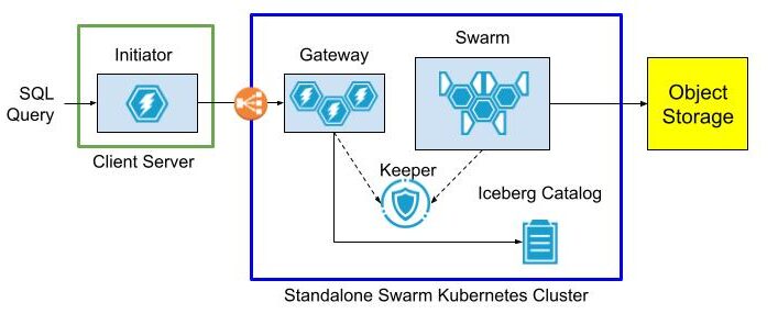
The gateway cluster has database definitions to expose data lake tables as well as user accounts so that clients can connect from outside networks as long as they can see the load balancer. Internals of the swarm cluster routing as well as query settings are completely hidden.
The following diagram shows the query flow.

Initiator, gateway, and swarm are just roles. You can name the actual clusters and servers within them anything you want.
Standalone Swarm Implementation
So much for theory. Let’s set up the standalone swarm.
Service Setup Overview
Our standalone swarm cluster is implemented in Kubernetes with the following services. For best results they should be based on the latest Antalya build.
- Antalya gateway cluster with at least one ClickHouse node.
- Antalya swarm cluster with auto-registration.
- Keeper ensemble.
- Altinity Ice REST Catalog.
Here are two ways to implement the configuration.
Method 1: Open Source
Follow the implementation procedure in https://github.com/Altinity/antalya-examples/tree/main/kubernetes. It sets up all required services, including the Iceberg REST catalog. The example uses the name “Vector” for the gateway cluster. Expose the Vector cluster and Ice REST Catalog load balancer ports. (E.g, by port forwarding as described in the README.md or by configuring public load balancers that expose access to Antalya servers and the Ice REST endpoint.)
Method 2: Altinity.Cloud
The other way is to set up all Standalone Swarm services in Altinity.Cloud. The Altinity Cloud Manager (ACM) documentation takes you through the easy process of creating clusters and swarm clusters. Use the latest Antalya builds for both gateway and swarm clusters.
- Using the ACM, create or get access to an Altinity.Cloud environment and open the Clusters tab.
- Use the LAUNCH CLUSTER function to start a gateway cluster with at least one available node. The examples that follow call this cluster my-gateway.
- Use the LAUNCH SWARM function to start a swarm cluster with at least one available node. The examples that follow call this cluster my-swarm.
- Ensure that your Altinity.Cloud environment has a configured Iceberg REST Catalog. We’ll read data from tables listed in this catalog. You can access the REST Catalog externally using connection details available in Altinity.Cloud. (Locate the Environment that contains your Antalya clusters.)
Configure Gateway Cluster for External Access
To access our standalone swarm, we’ll need to define a ClickHouse login with settings to access the swarm for queries. These settings are hidden to applications that connect to the gateway. First, add a user with privileges on the swarm.
-- RBAC setup for swarm user. Apply to gateway server(s).
DROP SETTINGS PROFILE IF EXISTS swarm_exec_profile ON CLUSTER '{cluster}';
DROP ROLE IF EXISTS swarm_exec_role ON CLUSTER '{cluster}';
DROP USER IF EXISTS swarm_exec_user ON CLUSTER '{cluster}';

-- Set the swarm cluster name and create a read-only role for queries.
CREATE SETTINGS PROFILE swarm_exec_profile ON CLUSTER '{cluster}'
SETTINGS
  object_storage_cluster = 'my-swarm'
READONLY;

CREATE ROLE swarm_exec_role ON CLUSTER '{cluster}'
  SETTINGS PROFILE 'swarm_exec_profile';

REVOKE ON CLUSTER '{cluster}' ALL FROM swarm_exec_role ;
GRANT ON CLUSTER '{cluster}' SELECT ON *.* TO swarm_exec_role;

-- Create a user with the above role.
CREATE USER swarm_exec_user ON CLUSTER '{cluster}'
  IDENTIFIED WITH SHA256_PASSWORD BY 'topsecret'
  HOST ANY
  DEFAULT ROLE swarm_exec_role;
Set Up Databases on the Gateway Cluster
Any table that we want to query needs to be visible on the gateway cluster. The simplest way is to add a database definition like the following.
CREATE DATABASE IF NOT EXISTS ice ON CLUSTER '{cluster}'
  ENGINE = DataLakeCatalog('https://iceberg-catalog.my-environment.altinity.cloud')
  SETTINGS catalog_type = 'rest',
    auth_header = 'Authorization: Bearer someToken',
    warehouse = 's3://my-bucket';
If you are an Ice Rest Catalog managed by Altinity.Cloud, you can get the connection URL, auth_header, and warehouse values by opening the environment that hosts your standalone cluster and selecting the Catalogs tab. (Contact your Org Admin if you cannot access this tab.)
Testing The Standalone Swarm
Let’s check the standalone swarm set to ensure it’s ready for use. First, we connect with our new account on the query gateway cluster.
Next we run queries to check that tables are visible and that we can issue a query on one of them. If your catalog has tables and access is properly configured you will see something like this:
SHOW TABLES FROM ice

   ┌─name─────────────────────────────────┐
1. │ aws-public-blockchain.btc            │
2. │ aws-public-blockchain.btc_live       │
3. │ aws-public-blockchain.btc_ps_by_date │
4. │ default.ontime                       │
5. │ ssb.lineorder_wide                   │
   └──────────────────────────────────────┘

SELECT count(), Carrier FROM ice.`default.ontime`
GROUP BY Carrier ORDER BY Carrier ASC

    ┌─count()─┬─Carrier─┐
 1. │ 3805480 │ AA      │
 2. │  455873 │ AL      │
 3. │  597874 │ AS      │
 4. │ 2125898 │ CO      │
 5. │ 3986228 │ DL      │
. . .
    └─────────┴─────────┘
The standalone swarm is ready for use.
Configure The Initiator ClickHouse Server
Add Cluster Definition for the Gateway
To use ClickHouse with our standalone swarm we need to do a bit of setup. First, let’s add a cluster definition to the configuration with the host, port, and credentials of the gateway cluster. Place the contents in /etc/clickhouse-server/config.d/swarm.xml. Restart the server for the settings to take effect.
<clickhouse>
  <remote_servers>
    <swarm>
       <shard>
          <replica>
              <host>my-gateway.my-environment.altinity.cloud</host>
              <port>9440</port>
              <secure>1</secure>
              <user>swarm_exec_user</user>
              <password>topsecret</password>
           </replica>
       </shard>
    </swarm>
  </remote_servers>
</clickhouse>
We can now route queries to the remote swarm.
Set Up Proxy Table Definitions
The next step is to set up remote tables on the client ClickHouse server. We do this for each data lake table we want to query via the remote swarm. For this demonstration we’ll just use a single table. Connect to the client ClickHouse and issue the following commands.
CREATE DATABASE IF NOT EXISTS ice_remote_swarm;

CREATE TABLE ice_remote_swarm.`default.ontime`
AS cluster(`swarm`, `ice`, `default.ontime`)
Let’s test that we can access the table.
SELECT count() FROM ice_remote_swarm.`default.ontime`

   ┌──count()─┐
1. │ 25801548 │ -- 25.80 million
   └──────────┘

1 row in set. Elapsed: 0.239 sec.
The response is pretty quick. We’ll get back to that shortly.
Optional Configuration for Testing
At this point our initiator server can query data lake tables through the standalone swarm. In this article, however, we go one step further and configure the cluster to connect directly to Iceberg. That allows us to run an apples-to-apples comparison with routing queries through the standalone swarm. If you don’t want to perform such a test, skip this section.
Configure A Filesystem Cache for S3 Reads on Parquet
One more thing–we need to configure caching for Parquet data read from S3. The following configuration file defines a filesystem cache for that purpose. Add it to /etc/clickhouse-server/config.d/cache.xml and restart the ClickHouse server.
<clickhouse>
  <filesystem_caches>
    <parquet_cache>
      <path>/var/lib/clickhouse/parquet_cache</path>
      <max_size>40Gi</max_size>
    </parquet_cache>
  </filesystem_caches>
</clickhouse>
You’ll need to ensure that the following settings are enabled to use the cache.
enable_filesystem_cache = 1
filesystem_cache_name = 'parquet_cache'
You can assign the values in a settings profile (XML or in SQL) or by appending them to queries after the SETTINGS keyword. (See below for more on the latter approach.)
Configure Direct Access to Data Lake
Finally we need to add a database definition that points to the Iceberg REST catalog.
CREATE DATABASE IF NOT EXISTS ice ON CLUSTER '{cluster}'
  ENGINE = DataLakeCatalog('https://iceberg-catalog.my-environment.altinity.cloud')
  SETTINGS catalog_type = 'rest',
    auth_header = 'Authorization: Bearer someToken',
    warehouse = 's3://my-bucket';
Let’s confirm that direct queries on the data lake work.
SELECT count()
FROM ice_direct.`default.ontime`

   ┌──count()─┐
1. │ 25801548 │ -- 25.80 million
   └──────────┘

1 row in set. Elapsed: 1.045 sec.
At this point all is in readiness. Time for some tests.
Testing The Standalone Swarm
Test Procedure
We can now measure the performance of the standalone swarm and compare it to reading data lake files directly from the client ClickHouse server. We use the following test query to look for Carriers with the worst cancellation record in a single year. Here’s an example.
SELECT Carrier, toYear(FlightDate) AS Year,
    (sum(Cancelled) / count(*)) * 100. AS cancelled_pct
FROM ice_direct.`default.ontime`
GROUP BY Carrier, Year HAVING cancelled_pct > 1.
ORDER BY cancelled_pct DESC LIMIT 2

   ┌─Carrier─┬─Year─┬──────cancelled_pct─┐
1. │ EA      │ 1989 │ 10.321500966388536 │
2. │ UA      │ 1992 │ 2.4398772291075796 │
   └─────────┴──────┴────────────────────┘
It’s not a big query and the dataset we’re using is relatively small (25M rows). However it’s enough to see basic behavior.
We run the test using a laptop that is running a local Client Server as shown above. The full test rig is shown below:
- Client Server Host – A Dell XPS 15 with Intel(R) Core(TM) i7-13700H, 32 GiB RAM, SSD drive. Win 11 Pro with ClickHouse running on WSL2.
- Gateway Cluster – A single AWS m8g.xlarge VM with 14 GiB RAM and 4 vCPUs allocated to ClickHouse.
- Swarm Cluster – 2 AWS m8g.xlarge VM with 14 GiB RAM and 4 vCPUs allocated to ClickHouse.
The standalone swarm is located in AWS US-East-1. The laptop is operating from California on a Comcast Internet connection measured at 415 Mbps download and 38.61 Mbps upload. (Pretty good connectivity by US standards.)
Here’s how we run the test.
- Clear caches on all hosts, including the local Client Server and all servers in the remote swarm. The commands to clear caches are the following.
SYSTEM DROP ICEBERG METADATA CACHE ON CLUSTER '{cluster}';
SYSTEM DROP FILESYSTEM CACHE ON CLUSTER '{cluster}';
SYSTEM DROP PARQUET METADATA CACHE ON CLUSTER '{cluster}';- Run queries 5 times for each of the following scenarios.
- Laptop directly to Iceberg using table ice_direct.`default.ontime` without caching enabled for S3, Iceberg metadata, or Parquet performance. This shows worst case performance on the laptop.
- Laptop directly to Iceberg using table ice_direct.`default.ontime` with caching enabled. This shows best case performance on the laptop.
- Laptop to the standalone swarm (through the proxy table ice_swarm.`default.ontime`).
In case you are wondering how to manage settings, the simplest way for testing is to turn them on and off explicitly. Here’s an example with all caches on.
SELECT Carrier, toYear(FlightDate) AS Year,
    (sum(Cancelled) / count(*)) * 100. AS cancelled_pct
FROM ice_direct.`default.ontime`
GROUP BY Carrier, Year HAVING cancelled_pct > 1.
ORDER BY cancelled_pct DESC LIMIT 2
SETTINGS enable_filesystem_cache = 1,
  filesystem_cache_name = 'parquet_cache',
  use_iceberg_metadata_files_cache = 1,
  input_format_parquet_use_metadata_cache = 1;
To turn them off, flip the 1’s to 0’s. Not pretty but it does the job.
Performance Test Results
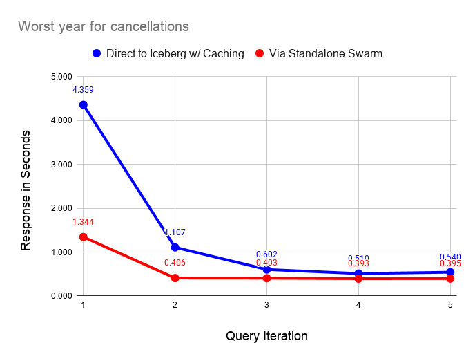
The following graph compares performance of direct query on the data lake with caches enabled versus the standalone swarm. As we can see, query on the standalone swarm is faster in all cases, but performance converges as caches fill on the laptop. As long as the dataset is small and can fit in laptop caches, the difference in response narrows significantly after running a couple of queries.
The following graph performs the same test as before but with all caching disabled on the laptop server. As before, querying via the swarm is faster in all cases. The interesting feature of this graph is the instability of reading from the data lake, even on a fast home Internet connection.

Ping times on the Internet connection are quite stable, which means that small requests go through quickly and reliably. However, the response on downloads from S3 is quite variable. The queries are pulling 111 MiB of data from S3 as shown by the following query on the filesystem cache size after a test run.
SELECT
    cache_name,
    formatReadableSize(sum(size)) AS size
FROM system.filesystem_cache
GROUP BY cache_name

   ┌─cache_name────┬─size───────┐
1. │ parquet_cache │ 111.24 MiB │
   └───────────────┴────────────┘
I ran these tests a couple of dozen times and found that the uncached response varied between 2 and 10 seconds. By contrast the standalone swarm returns query results in 0.4 seconds once caches fill with relatively little variance across runs. The data shared across the Internet connection is very small in the latter case, since scanning and aggregation occurs on the standalone swarm.
It’s also important to note that the dataset we are querying is also quite small, hence shows the laptop performance in a favorable light. The standalone swarm performance looks vastly better as the dataset size increases. You would not want to use direct query from the laptop in this case.
Using Standalone Swarms With Non-Antalya Servers
As we mentioned in the introduction, standalone swarms can accelerate data lake queries on any ClickHouse version. Let’s demonstrate this with clickhouse-local using the latest upstream Official ClickHouse build. It won’t take long.
Start by installing Official ClickHouse. I love this quick download with curl. It’s the handiest database installation of all time.
curl https://clickhouse.com/ | sh
. . .
Successfully downloaded the ClickHouse binary, you can run it as:
    ./clickhouse
Now start clickhouse-local.
./clickhouse local
Decompressing the binary......
ClickHouse local version 26.3.1.357 (official build).
…And run a query directly against the standalone swarm. The call to remoteSecure() feels a little hacky but we’re moving fast and breaking things. Elegance can come later.
:) SELECT Carrier, toYear(FlightDate) AS Year,
    (sum(Cancelled) / count(*)) * 100. AS cancelled_pct
FROM remoteSecure('my-gateway.my-environment.altinity.cloud:9440', ice, 'default.ontime', 'swarm_exec_user', 'topsecret')
GROUP BY Carrier, Year HAVING cancelled_pct > 1.
ORDER BY cancelled_pct DESC LIMIT 2

   ┌─Carrier─┬─Year─┬──────cancelled_pct─┐
1. │ EA      │ 1989 │ 10.321500966388536 │
2. │ UA      │ 1992 │ 2.4398772291075796 │
   └─────────┴──────┴────────────────────┘

2 rows in set. Elapsed: 1.097 sec. Processed 25.80 million rows, 365.33 MB (23.53 million rows/s., 333.17 MB/s.)
Peak memory usage: 26.18 MiB.
Q.E.D. This query should work with any version of ClickHouse, but note that the query host nam is not real.
For now, you need to set up your own standalone swarm cluster as described above. We’re building a Project Antalya public demo environment that you will be able to use from any location. It should be out in a few weeks.
Conclusion
Standalone swarm clusters are a neat variation on Antalya swarms that allow any ClickHouse server to accelerate queries on data lakes. Standalone swarms are (a) movable and (b) completely encapsulate swarm hosts, settings, and cache configuration for high performance. For this reason standalone swarms can also eliminate transfer costs from public clouds.
There’s more to come. Standalone swarms are a linchpin that makes it easier to extend existing ClickHouse tables onto cheap Iceberg storage using Antalya Hybrid tables. We will expand on this important use case shortly in a new blog article that will appear shortly.
Modern data lakes open up exciting new possibilities for cheap, real-time analytics. We hope you have enjoyed this article and that it inspires you to create new applications with Project Antalya. If you need help, please contact us or join our Slack workspace to ask questions.
The post Data Lake Query Acceleration using Standalone Antalya Swarms appeared first on Altinity | Run open source ClickHouse® better.
]]>The post Altinity Stable Build for ClickHouse® 25.8 appeared first on Altinity | Run open source ClickHouse® better.
]]>Version 25.8 Release Summary
Development always moves fast in the ClickHouse GitHub project. More than 300 contributors from companies all around the world submitted 3200+ pull requests with new features and improvements. We spent several months testing the new version and tracking fixes merged to the 25.8 LTS branch. We also collected early adopter feedback on upgrades as well as feature changes that affect production use.
One example of that is the high memory usage due to very wide system tables. Another detective story was a broken DDL worker that affected many new Docker and Kubernetes deployments. Now that they are fixed, we are confident in certifying 25.8 as ready for use.
Detailed release notes for Altinity Stable Build 25.8 are available on the Altinity Documentation Site. There are a lot of new features, but also many behavior changes, so check the release notes carefully before upgrading.
Differences Between Altinity Stable Builds and Upstream Official Builds
Like upstream builds, Altinity Stable builds for ClickHouse are open source and are based on upstream LTS versions. Altinity Stable Build version 25.8.16.10001 is based on upstream 25.8.16.34-lts, but we have additionally backported several fixes from newer versions:
- ALTER MODIFY COLUMN now requires explicit DEFAULT when converting nullable columns to non-nullable types. Previously such ALTERs could get stuck with cannot convert null to not null errors. Now NULLs are replaced with column’s default expression (ClickHouse#84770 by @vdimir via #1344)
- Added new SQL statement EXECUTE AS to support user impersonation (ClickHouse#70775 by @shiyer7474, ClickHouse#90437 by @alexbakharew via #1340)
- Fix crash in StorageDistributed when parsing malformed shard directory names (ClickHouse#90243 by @AVMusorin via #1343)
- Datalake catalogs will be shown in system introspection tables only if
show_data_lake_catalogs_in_system_tablesexplicitly enabled (ClickHouse#88341 by @alesapin via #1331) - ClickHouse will show data lake catalog database in SHOW DATABASES query by default (ClickHouse#89914 by @alesapin via #1331)
- Possible crash/undefined behavior in IN function where primary key column types are different from IN function right side column types (ClickHouse#89367 by @ilejn via #1339)
- Fixed move-to-prewhere optimization, which did not work in the presence of row policy (ClickHouse#87303 by @KochetovNicolai via #1345)
- Fixes a bug where certain distributed queries with ORDER BY could return ALIAS columns with swapped values (i.e., column a showing column b’s data and vice versa) (ClickHouse#94644 by @filimonov via #1346)
- Split part ranges by volume characteristics to enable TTL drop merges for cold volumes. After this patch, parts with a max TTL < now will be removed from cold storage. The algorithm will schedule only single part drops. (ClickHouse#90059 by @Michicosun via #1363)
- Check and mark the interserver IP address active in DDL worker (ClickHouse#92339 by @tuanpach via #1403)
- Fix handling of users with a dot in the name when added via config file (ClickHouse#86633 by @mkmkme via #1342)
- S3Queue auxiliary Zookeeper support using
keeper_pathsetting from s3Queue (ClickHouse#95203 by @lesandie via #1357) - SELECT query with FINAL clause on a ReplacingMergeTree table with the is_deleted column now executes faster because of improved parallelization from 2 existing optimizations (ClickHouse#88090 by @shankar-iyer via #1332)
- Reduce INSERT/merges memory usage with wide parts for very wide tables by enabling adaptive write buffers. Add support of adaptive write buffers for encrypted disks (ClickHouse#92250 by @azat via #1341)
We have also disabled one setting to allow safe downgrade from 25.8 to 25.3:
- Disable
write_marks_for_substreams_in_compact_partsby default to preserve downgrade compatibility (#1407 by @zvonand)
Let’s Install!
Altinity Stable build packages for different Linux distributions can be found at https://builds.altinity.cloud.
Altinity Stable build container images are available as altinity/clickhouse-server:25.8.16.10001.altinitystable on Docker Hub.
Altinity.Cloud users may upgrade to a new build using Cluster Upgrade wizard.
For more information on installing Altinity Builds, see the Altinity Stable® Builds Install Guide. Please contact us at [email protected] if you experience any issues with the upgrade.
Project Antalya or Altinity Stable?
Altinity Stable builds are focused on safe upgrades and stability for production operation. If you are interested in the newest features for data lakes, Iceberg, Parquet and other cool stuff, try out Project Antalya builds. Those represent the latest Altinity work on the Project Antalya.
Want More Information About Altinity Stable Builds?
Check out our blog article on the upgrade philosophy behind Altinity Stable Builds and how it differs from official ClickHouse builds. Altinity supports both builds, so you can choose whichever is best for you!
The post Altinity Stable Build for ClickHouse® 25.8 appeared first on Altinity | Run open source ClickHouse® better.
]]>The post Navigating Object Storage and Iceberg Data Lakes with ClickHouse® SQL appeared first on Altinity | Run open source ClickHouse® better.
]]>We’ll prove the point by using ClickHouse SQL to examine every aspect of an Iceberg table, from enumeration of files to queries on Iceberg REST catalogs. The Iceberg table format is a perfect example to show off ClickHouse capabilities. Iceberg tables have complex metadata and multiple file types. With simple SQL queries, the information becomes easily visible.
This capability is useful for many reasons, of which two are especially important. First, many applications write and read data in Iceberg tables. It’s important to be able to examine tables directly when debugging problems, optimizing performance, or just trying to understand what’s there. Second, ClickHouse SQL is a great foundation for tools that manage Iceberg tables. There’s no reason to bring in extra tools outside the database. You can build on ClickHouse.
How Are Iceberg Tables Structured?
Let’s start with a quick primer on Apache Iceberg table structure. This will help readers understand how things are put together. Iceberg files are generally loaded using a path that includes the table name and divides into separate paths for data and metadata. It looks like the following.

These are conventions, and not every Iceberg table follows them. It depends on the tool used to write the table as well as user choices. For example, it’s possible to put data files under a different path from metadata files. You can also add additional files. Dremio and some other implementations add a file named version-hint.text to locate the latest table version. Finally there’s no hard and fast rule for naming files. Instead, we locate files by reading the Iceberg table metadata, not by their names.
The files we are touring in this article were exported from ClickHouse using the new Project Antalya ALTER TABLE EXPORT COMMAND. I imported them into Iceberg using the Altinity Ice utility invoked as follows. The command specifies the partitioning and sort order. We will see this information in the Iceberg metadata data.
ice insert default.ontime -p --thread-count=12 \
 --no-copy \
 --partition='[{"column":"Year"}]' \
 --sort='[{"column":"Carrier", "desc":false}, {"column":"FlightDate", "desc":false}]' \
 --assume-sorted \
"s3://my-bucket/default/ontime/data/*/*.parquet"
Finding Out What’s in Object Storage
Let’s start with the basics: files on S3 object storage. Speaking of which, what files are in our Iceberg table? We can start with a simple query to enumerate the full path of each file.
SELECT _path
FROM s3('s3://my-bucket/default/ontime/**', One)
ORDER BY _path ASC FORMAT Vertical

Row 1:
──────
_path: my-bucket/default/ontime/data/Year=1987/1987_1_1_0_EBFB...C1C4.1.parquet
Row 2:
──────
_path: my-bucket/default/ontime/data/Year=1987/1987_3_3_0_E995...6C1.1.parquet
Row 3:
──────
_path: my_bucket/default/ontime/data/Year=1987/commit_1987_1_1_0_EBF...C1C4
Our query uses the s3() table function and leans on three key features to extract relevant information.
- Virtual columns. The _path column gives the full path to the file in object storage.
- Wildcards. The ‘**” wildcard matches any file that starts with the prefix.
- The One input format. This is a special format that reads file metadata only, not the rows inside it. The result is one output row for each file.
We can add more virtual columns to get additional metadata. Here is a query showing all of those supported for files in S3.
SELECT _path, _file, _size, _time, _etag
FROM s3('s3://my-bucket/default/ontime/data/Year=1987/1987_1_1_0_EBFB...C1C4.1.parquet', One)
FORMAT Vertical

Row 1:
──────
_path: my-bucket/default/ontime/data/Year=1987/1987_1_1_0_EBFB...C1C4.1.parquet
_file: 1987_1_1_0_EBFB...C1C4.1.parquet
_size: 12257633 -- 12.26 million
_time: 2026-02-21 12:50:44
_etag: "58c79fbcd1dd8a0b850ae10293bdc905"
Here’s a quick summary of each virtual column derived from reading ClickHouse source code. (The docs were ambiguous. Thanks for helping, Claude!)
| Virtual Column | Description |
| _path | Full path to file |
| _file | Filename only (without directory path) |
| _size | File size in bytes |
| _time | Last modified time |
| _etag | ETag (entity tag) of the file, which is a hash of the stored object |
We can also gather file data in a more succinct form using aggregation. How many file types are in the table and how many files does each one have? Here is the query to find out.
SELECT extract(_file, '.*\\.(.*)$') AS file_type, count()
FROM s3('s3://my-bucket/default/ontime/**', One)
GROUP BY file_type
ORDER BY file_type ASC

   ┌─file_type─┬─count()─┐
1. │           │      13 │
2. │ avro      │       2 │
3. │ json      │       2 │
4. │ parquet   │      13 │
   └───────────┴─────────┘
This is interesting. What are the files without data types? It turns out they are generated during export of parts from ClickHouse to S3 object storage. They aren’t part of the Iceberg format, and the Altinity Ice Catalog will eventually clean them up automatically as part of table maintenance. Let’s see what’s in one of them.
SELECT * FROM s3('s3://my-bucket/default/ontime/data/Year=1987/commit_1987_3_3_0_E995...F6C1')

Row 1:
──────
default/ontime/data/Year: 1987/1987_3_3_0_E995...F6C1.1.parquet
Year:                     1987
We see the data, but what kind of file are we looking at? ClickHouse does not give up this secret easily. However, if you add SETTINGS send_logs_level = ‘debug’ to the query and search the resulting log messages, you’ll find that it is the TSKV input format. The clickhouse-client output is shown below.
SELECT * FROM s3('s3://my-bucket/default/ontime/data/Year=1987/commit_1987_3_3_0_E995...F6C1')
SETTINGS send_logs_level = 'debug'
. . .
[chi-my-swarm-my-swarm-0-0-0] 2026.02.24 16:10:08.342674 [ 806 ]  {dab4f667-b89d-49d2-9f56-e10810779f95} <Debug> executeQuery: (from [::ffff:10.129.152.255]:34032, user: swarm_access, initial_query_id: 138bb6df-afbe-4e87-82c6-3a9fa8172122) (query 1, line 1) SELECT __table1.`default/ontime/data/Year` AS `default/ontime/data/Year`, __table1.Year AS Year FROM s3Cluster('my-swarm', 's3://my-bucket/default/ontime/data/Year=1987/commit_1987_3_3_0_E9959EB7178905EA836AFB9D8645F6C1', 'TSKV', '`default/ontime/data/Year` Nullable(String), `Year` Int64') AS __table1 SETTINGS send_logs_level = 'debug' (stage: WithMergeableState)
(I said ClickHouse does not give up the secret easily!)
The fact you can read file data without even knowing the format is incredibly handy. ClickHouse’s ability to handle different file formats automatically is quite amazing.
Let’s move up a level and ask one more question. We have the path to one Iceberg table already. Are there others in the bucket? We can find out with a bit of regular expression hackery. There are five tables.
SELECT DISTINCT arrayStringConcat(table_array, '.') AS table_name
FROM
(
    SELECT
        extract(_path, '[a-zA-Z0-9]*/(.*)/metadata/.*$') AS table_path,
        splitByChar('/', table_path) AS table_array
    FROM s3('s3://my-bucket/**', One)
    WHERE length(table_path) > 0
)
ORDER BY table_name ASC

   ┌─table_name───────────────────────────┐
1. │ aws-public-blockchain.btc            │
2. │ aws-public-blockchain.btc_live       │
3. │ aws-public-blockchain.btc_ps_by_date │
4. │ default.ontime                       │
5. │ ssb.lineorder_wide                   │
   └──────────────────────────────────────┘
One final note! If you are using a Project Antalya build, you should know about the use_object_storage_list_objects_cache setting. It caches calls to enumerate lists of files on S3-compatible storage. This speeds up queries on buckets with many files substantially but means you may not see recently added files. If you think this is happening you can turn it off as shown in the following example.
SELECT DISTINCT _path, _file, _size, _time, _etag
FROM s3('s3://my-bucket/default/ontime/**', One)
SETTINGS use_object_storage_list_objects_cache = 0
Looking at Parquet File Data and Metadata
Our Iceberg table stores data in Parquet files, the most popular columnar file format for data lakes. Parquet format is fully documented here, in case you want to do some background reading. Meanwhile, ClickHouse can help us learn about what’s inside individual Parquet files very quickly. For example, we can count the rows as follows. In fact this file is just like a SQL table. You can run any query on it you like.
SELECT count() FROM s3('s3://my-bucket/default/ontime/data/Year=1993/1993_37_37_0_8532...9889.1.parquet')

   ┌─count()─┐
1. │  740075 │
   └─────────┘
Just like a SQL table we can also describe the Parquet file columns.
DESCRIBE TABLE s3('s3://my-bucket/default/ontime/data/Year=1993/1993_37_37_0_8532...9889.1.parquet')
FORMAT Vertical

Row 1:
──────
name:               Year
type:               Nullable(UInt16)
...
It’s convenient that ClickHouse fetches the type information but we can also get it directly from the Parquet file. The format is fully self-describing and the following query dumps everything.
SELECT *FROM s3('s3://my-bucket/default/ontime/data/Year=1993/1993_37_37_0_8532...9889.1.parquet', ParquetMetadata)The ParquetMetadata input format is a key piece of magic that makes the queries work. It dumps the metadata from Parquet instead of the data. Unfortunately, the result is an ugly mess with nested definitions of columns and row groups. Fortunately, it only takes a small effort to make the output more civilized.
First, let’s let ClickHouse describe the complete format of the metadata. It will even show nested data structures.
DESCRIBE TABLE s3('s3://my-bucket/default/ontime/data/Year=1993/1993_37_37_0_8532...9889.1.parquet', ParquetMetadata)

Row 1:
──────
name:               num_columns
type:               UInt64
. . .
Once we have names for columns and the nested structures within them, it’s possible to create queries that make things human readable. Let’s start with general information about the Parquet file contents.
SELECT
    _file, num_columns, num_rows, num_row_groups,
    format_version, total_uncompressed_size, total_compressed_size
FROM s3('s3://my-bucket/default/ontime/data/Year=1993/1993_37_37_0_8532...9889.1.parquet', ParquetMetadata)
FORMAT Vertical

Row 1:
──────
_file:                   1993_37_37_0_8532...9889.1.parquet
num_columns:             109
num_rows:                740075
num_row_groups:          1
format_version:          2
total_uncompressed_size: 25352826 -- 25.35 million
total_compressed_size:   10847364 -- 10.85 million
Next, let’s look at the column definitions. Thanks to the handy ARRAY JOIN operation we can unroll the nested column definitions.
SELECT
    col.name AS name,
    col.physical_type AS physical_type,
    col.logical_type AS logical_type,
    col.compression AS compression,
    col.total_uncompressed_size AS total_uncompressed_size,
    col.total_compressed_size AS total_compressed_size,
    col.space_saved AS space_saved,
    col.encodings AS encodings
FROM s3('s3://my-bucket/default/ontime/data/Year=1993/1993_37_37_0_8532...9889.1.parquet', ParquetMetadata)
ARRAY JOIN columns AS col
FORMAT Vertical

Row 1:
──────
name:                    Year
physical_type:           INT32
logical_type:            Int(bitWidth=16, isSigned=false)
compression:             ZSTD
total_uncompressed_size: 69
total_compressed_size:   101
space_saved:             -46.38%
encodings:               ['PLAIN','RLE_DICTIONARY']
. . .
If you like to nerd out on data types, this is gold. It’s beautiful to see that Parquet supports unsigned integer types. It also defaults (in this case) to ZSTD compression.
Parquet stores data in row groups, which are sets of rows in columnar format. They are like granules in ClickHouse MergeTree tables. We can get exact information about each row group.
SELECT
    rg.file_offset AS file_offset,
    rg.num_columns AS num_columns,
    rg.num_rows AS num_rows,
    rg.total_uncompressed_size AS total_uncompressed_size,
    rg.total_compressed_size AS total_compressed_size
FROM s3('s3://my-bucket/default/ontime/data/Year=1993/1993_37_37_0_8532...9889.1.parquet', ParquetMetadata)
ARRAY JOIN row_groups AS rg
FORMAT Vertical

Row 1:
──────
file_offset:             4
num_columns:             109
num_rows:                740075
total_uncompressed_size: 25352826 -- 25.35 million
total_compressed_size:   10847364
Our file is small so there is just one row group. We can even reach into the row group and get information about each column in the group, such as the min and max values of the column. Here’s how to do it.
SELECT
    file_offset AS offset, col.name AS name,
    col.statistics.min AS min, col.statistics.max AS max
FROM
(
    SELECT
        rg.file_offset AS file_offset,
        rg.columns AS columns
    FROM s3('s3://my-bucket/default/ontime/data/Year=1993/1993_37_37_0_8532...9889.1.parquet', ParquetMetadata)
    ARRAY JOIN row_groups AS rg
)
ARRAY JOIN columns AS col

     ┌─offset─┬─name─────────────────┬─min──────────────┬─max──────────────┐
  1. │      4 │ Year                 │ 1993             │ 1993             │
  2. │      4 │ Quarter              │ 1                │ 4                │
  3. │      4 │ Month                │ 1                │ 12               │
  4. │      4 │ DayofMonth           │ 1                │ 31               │
  5. │      4 │ DayOfWeek            │ 1                │ 7                │
  6. │      4 │ FlightDate           │ 8401             │ 8765             │
. . .
At this point we’ve learned a great deal about the Parquet file contents, and further inquiry might exceed the bounds of good taste. The metadata is now at your disposal. We’ll meanwhile turn to look at Iceberg table metadata.
Finding Out What’s in an Iceberg Table
Iceberg metadata is stored in a combination of JSON and Avro files. Let’s trace through and see what’s inside. To make the results easier to understand, we’ll first start by showing how the metadata files are related. This is a simpler version of the picture provided by the Iceberg specification that uses real file names.
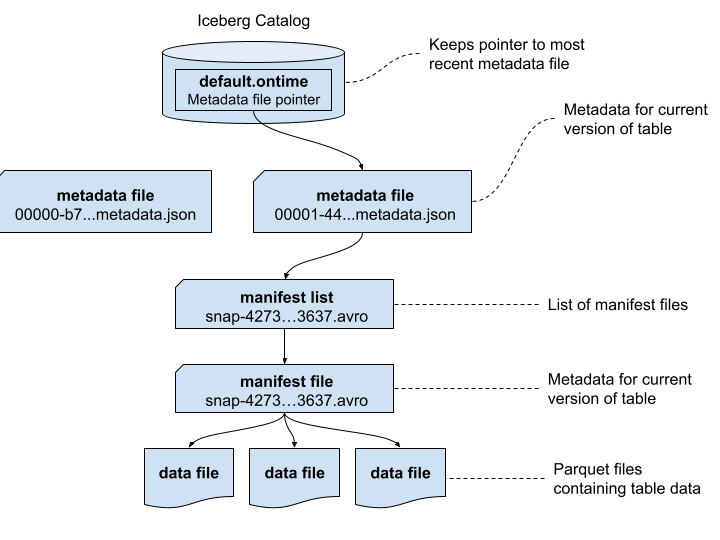
It’s a good time to point out that the Apache Iceberg project provides a full table specification that covers the contents of each of the above files, including precise definitions of each field. Many fields are self-explanatory, but if in doubt you now have a source for full answers.
Let’s first start by enumerating the metadata files. We will also sort them by descending time.
SELECT
    _path,
    _time
FROM s3('s3://my-bucket/default/ontime/metadata/**', One)
ORDER BY _time DESC
FORMAT Vertical

Row 1:
──────
_path: my-bucket/default/ontime/metadata/00001-4457...6779.metadata.json
_time: 2026-02-21 14:08:47

Row 2:
──────
_path: my-bucket/default/ontime/metadata/snap-4273...3637.avro
_time: 2026-02-21 14:08:46
. . .
Next, we want to find the schema of the metadata.json files using the last file written. (If you pick the first file there is a chance it may not contain all schema, because it may not have any manifests yet.)
DESCRIBE s3('s3://my-bucket/default/ontime/metadata/00001-4457...6779.metadata.json')
FORMAT Vertical
Let’s run a query to check the main properties of the table. We won’t bother to unroll the nested structures like partition specs and sort orders. Instead, we can print them in prettified JSON, which is quite readable.
SELECT
    `format-version`,
    location,
    `last-sequence-number`,
    `last-updated-ms`,
    `partition-specs`,
    `sort-orders`
FROM s3('s3://my-bucket/default/ontime/metadata/00001-4457...6779.metadata.json')
FORMAT PrettyJSONEachRow

{
    "format-version": 2,
    "location": "s3:\/\/my-bucket\/default\/ontime",
    "last-sequence-number": 1,
    "last-updated-ms": 1771682926743,
    "partition-specs": [
        {
            "fields": [
                {
                    "field-id": 1000,
                    "name": "Year",
                    "source-id": 1,
                    "transform": "identity"
                }
                ...
It’s more interesting to unroll the column definitions into a proper table. Here’s a query to do that.
SELECT
    field.id AS id,
    field.name AS name,
    field.required AS required,
    field.type AS type
FROM s3('s3://my-bucket/default/ontime/metadata/00001-4457...6779.metadata.json')
ARRAY JOIN tupleElement(schemas[1], 'fields') AS field
ORDER BY id ASC

     ┌──id─┬─name─────────────────┬─required─┬─type─────┐
  1. │   1 │ Year                 │ true     │ int      │
  2. │   2 │ Quarter              │ true     │ int      │
  3. │   3 │ Month                │ true     │ int      │
  4. │   4 │ DayofMonth           │ true     │ int      │
  5. │   5 │ DayOfWeek            │ true     │ int      │
  6. │   6 │ FlightDate           │ true     │ date     │
  . . .
This query works if you don’t change the schema, in which case there is just one set of columns However, if the schema *does* change there will be multiple schemas and you might not get the right one. We’ll leave that as a challenge for energetic readers.
We can move away from the Iceberg schema to find out which files belong to the table. The first thing to do is find the manifest lists, which is exactly what this query does.
SELECT
    snap.`manifest-list` AS manifest_list,
    snap.`schema-id` AS schema_id,
    snap.`sequence-number` AS sequence_number,
    snap.`snapshot-id` AS snapshot_id
FROM s3('s3://my-bucket/default/ontime/metadata/00001-4457...6779.metadata.json')
ARRAY JOIN snapshots AS snap
FORMAT Vertical

Row 1:
──────
manifest_list:   s3://my-bucket/default/ontime/metadata/snap-4273...3637.avro
schema_id:       0
sequence_number: 1
snapshot_id:     4273857594351972880
The full path for the single manifest list is shown in the output. It’s encoded in Avro, which is a self-describing columnar format like Parquet. We can read the file contents as follows.
SELECT * FROM s3('s3://my-bucket/default/ontime/metadata/snap-42738...3637.avro')
FORMAT Vertical

Query id: d8c7f7be-910d-46f1-8c5f-236b244783dc

Row 1:
──────
manifest_path:        s3://my-bucket/default/ontime/metadata/e0ea...3637-m0.avro
manifest_length:      22087
partition_spec_id:    0
. . .
There is just one manifest file but it has a lot of nested information. We’ll read that using a query that breaks out the nested information in a more human-readable format.
SELECT status, snapshot_id, sequence_number, file_sequence_number,
  data_file.content AS content,
  data_file.file_path AS file_path,
  data_file.file_format AS file_format,
  data_file.partition AS partition
FROM
s3('s3://my-bucket/default/ontime/metadata/e0ea...3637-m0.avro')
FORMAT Vertical

Row 1:
──────
status:               1
snapshot_id:          4273857594351972880
sequence_number:      ᴺᵁᴸᴸ
file_sequence_number: ᴺᵁᴸᴸ
content:              0
file_path:            s3://my-bucket/default/ontime/data/Year=1987/1987_1_1_0_EBFB...C1C4.1.parquet
file_format:          PARQUET
partition:            (1987)
. . .
The manifest list is an interesting and critically important file. It provides statistics that ClickHouse uses to prune partitions and skip files within partitions. We can see already that our Parquet files are assigned to the expected partitions, which is comforting. Ensuring statistics are correct is a high priority so that queries run fast and return the right results.
Finally, we showed previously how to locate Iceberg tables using regex expressions on file names. We can also find the paths by scanning metadata.json files, as shown in the following example.
SELECT DISTINCT location
FROM s3('s3://my-bucket/**/*.metadata.json')
ORDER BY location
SETTINGS input_format_json_use_string_type_for_ambiguous_paths_in_named_tuples_inference_from_objects = 1
   ┌─location────────────────────────────────────────────┐
1. │ s3://my-bucket/aws-public-blockchain/btc_live       │
2. │ s3://my-bucket/default/ontime                       │
3. │ s3://my-bucket/aws-public-blockchain/btc            │
4. │ s3://my-bucket/aws-public-blockchain/btc_ps_by_date │
5. │ s3://my-bucket/ssb/lineorder_wide                   │
   └─────────────────────────────────────────────────────┘
Note the input_format_json_use_string_type_for_ambiguous_paths… setting on this query. Depending on their content metadata.json files may have different schemas. This setting tells ClickHouse to reconcile ambiguous paths in JSON. Without it your query may fail.
Working With Iceberg REST Catalogs
Not everything in Iceberg tables is a file in object storage. Iceberg REST catalogs track the current location of file metadata, which saves you from having to scan Iceberg metadata.json files to find the most current table snapshot.
We can query Iceberg REST catalogs using the ClickHouse url() functions. You’ll need to have a bearer token or another means of authentication to the catalog. Here’s an example of querying the available namespaces for Iceberg tables.
SELECT namespace
FROM url('http://ice-rest-catalog:5000/v1/namespaces', headers('Authorization' = 'Bearer someTokenString'))
ARRAY JOIN namespaces AS namespace

   ┌─namespace─────────────────┐
1. │ ['aws-public-blockchain'] │
2. │ ['default']               │
3. │ ['ssb']                   │
   └───────────────────────────┘
We can now query the tables within the default namespace.
SELECT
    `table`.name AS table_name,
    `table`.namespace AS table_namespace
FROM url('http://ice-rest-catalog:5000/v1/namespaces/default/tables', headers('Authorization' = 'Bearer someTokenString'))
ARRAY JOIN identifiers AS `table`

   ┌─table_name─┬─table_namespace─┐
1. │ ontime     │ ['default']     │
   └────────────┴─────────────────┘
Finally, we can look up the location of the current metadata.json file for the ontime table.
SELECT `metadata-location`
FROM url('http://ice-rest-catalog:5000/v1/namespaces/default/tables/ontime', headers('Authorization' = 'Bearer someTokenString'))
FORMAT Vertical

Row 1:
──────
metadata-location: s3://my-bucket/default/ontime/metadata/00001-4457...6779.metadata.json
There is much more information available from this last call. The REST response contains data from the metadata.json, so you don’t have to read the file directly. To see names of the available fields you can use the following handy DESCRIBE invocation.
DESCRIBE TABLE
(
    SELECT *
    FROM url('http://ice-rest-catalog:5000/v1/namespaces/default/tables/ontime', headers('Authorization' = 'Bearer someTokenString'))
)
For more information on Iceberg REST API calls, check out the official specification online.
Conclusion
ClickHouse SQL offers a comprehensive and flexible solution to reading both data as well as metadata from data lakes, including Iceberg tables. We’ve shown how ClickHouse can help you quickly understand the structure and data in Iceberg tables. Its ability to read complex structures across JSON, Avro, and Parquet using simple SQL queries is nothing short of amazing.
ClickHouse SQL is also a great basis for Iceberg table management tools, which can now operate without needing direct access to files, object storage, or Iceberg REST catalogs. We will illustrate some of the things you can build on this foundation in future blog articles.
If you have further questions about this article or any aspect of using ClickHouse with Iceberg data lakes, please contact us or join our Slack workspace to ask questions. We look forward to hearing from you.
The post Navigating Object Storage and Iceberg Data Lakes with ClickHouse® SQL appeared first on Altinity | Run open source ClickHouse® better.
]]>The post Using Altinity.Cloud to Log Sensor Data with ClickHouse® Endpoints appeared first on Altinity | Run open source ClickHouse® better.
]]>But keep your eye on the temperature and pressure.
-Seamus Heaney, The Cure at Troy
In an earlier blog post, we demonstrated how ClickHouse Endpoints can simplify your applications. The examples there exposed ClickHouse queries as REST endpoints, letting authenticated users run those queries and get the results without any knowledge of the queries themselves.
Those examples only used the GET verb. In this blog post, we’ll take a look at invoking a ClickHouse endpoint with a POST request. ClickHouse will take the data from the POST request and use it in an INSERT statement. Our scenario is that we have a BME680 temperature sensor attached to a single-board computer (SBC). There could be many of these devices in, for example, a warehouse. Each device can read its sensor and put together a POST request with the data from the sensor.
We tested the code on three devices: a Raspberry Pi Model 4B with 8GB RAM, a Raspberry Pi Zero 2 W, and a Raspberry Pi Pico W. The Raspberry Pis are SBCs that run Linux, while the Raspberry Pi Pico W is a microcontroller that runs MicroPython.
See the appendix for a list of the hardware we used.
Photos of These Machines at Work
To whet your appetite, we’ll look at pictures of these machines reading the sensor and sending data to ClickHouse. For the Raspberry Pis, your author configured ssh when burning the system image onto the Micro SD card so no keyboard, mouse, or monitor would be needed to work with the machine. The only thing plugged into the boards is the power supply.
Here’s the setup on a Raspberry Pi 4 Model B:

Figure 1. A Raspberry Pi 4B with a BME680 sensor attached
This features the Pimoroni BME680 breakout board with right-angle female headers. The Pimoroni board matches the pinouts for the Raspberry Pi, making it easy to connect.
The Pi Zero 2 W is similar, just smaller:

Figure 2. A Raspberry Pi Zero 2 W with a BME680 sensor attached
These two machines run the same code. As a final example, here’s a Raspberry Pi Pico W microcontroller inserting data into ClickHouse:
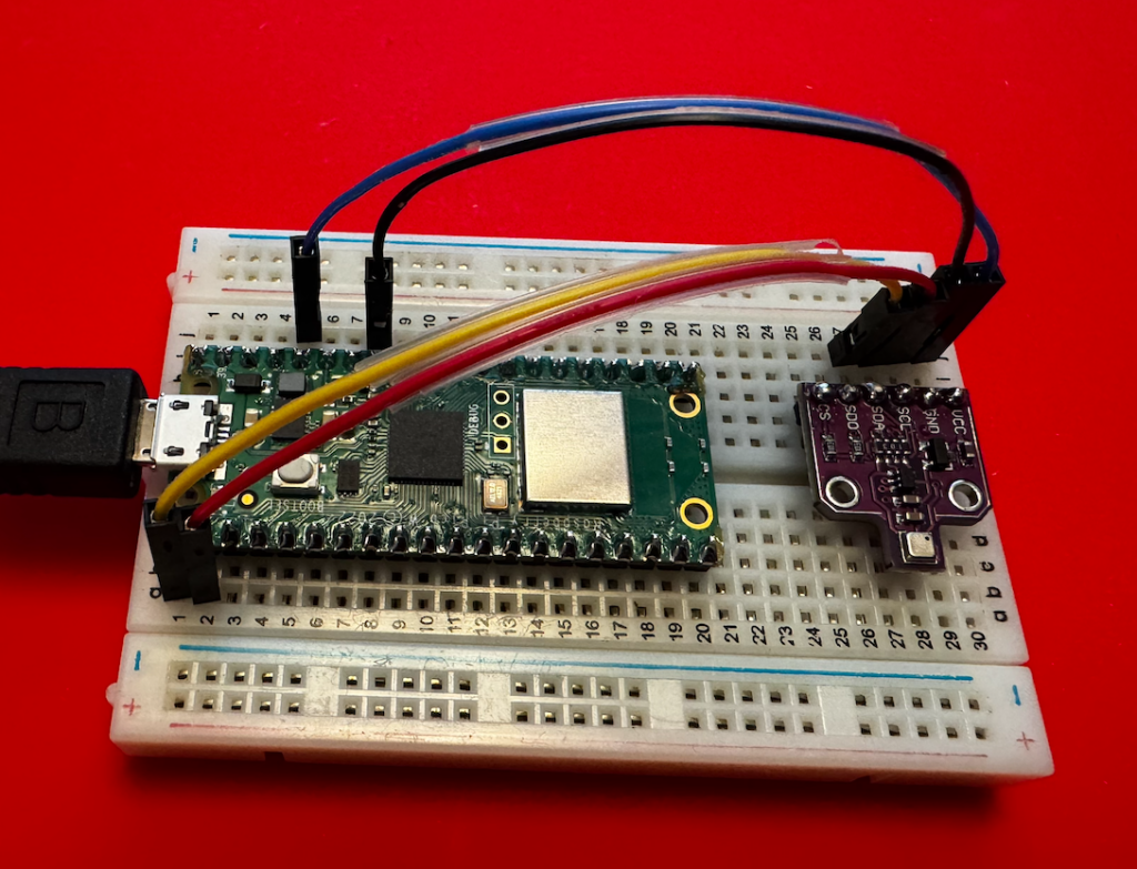
Figure 3. A Raspberry Pi Pico W wired to a BME680 sensor on a breadboard
The Pico doesn’t have an SD card, and it doesn’t run Linux; it runs MicroPython in its 264KB of RAM and 2MB of flash storage. (Yes, those numbers are kilobytes and megabytes.) When you power it on, it looks for main.py and runs it. And here we’re using a different breakout board for the BME680, with jumper wires connecting the correct pins from the Pico to the sensor.
But First…
We’ll look at how to set up the machines and run the code on them, but first we need a ClickHouse cluster and database and endpoint to store the data. So:
- If you don’t have an Altinity.Cloud account already, sign up for a free trial.
- Once you have an account, create a new ClickHouse cluster.
Creating Our Sample Database
Before we can create an API endpoint to our ClickHouse cluster, we need to create the database. Run this command to create it:
CREATE DATABASE IF NOT EXISTS maddie ON CLUSTER '{cluster}';
Now create the table:
CREATE TABLE maddie.sensor_data ON CLUSTER '{cluster}'
(
    time_stamp DateTime64(3),
    temp Float32,
    humidity Float32,
    pressure Float32,
    sensor String
)
ENGINE = ReplicatedMergeTree('/clickhouse/{cluster}/tables/maddie/sensor_data', '{replica}')
ORDER BY tuple()
SETTINGS index_granularity = 8192;
With the database in place, we’ll define a ClickHouse endpoint for our code to insert data.
Creating an Endpoint in the ACM
The API Endpoints tab is in the ACM’s Cluster Explorer. We’ll look at the UI of the endpoint editor to show you how easy it is to work with endpoints. When you open the tab for the first time, you’ll see this:

Figure 4. No ClickHouse endpoints defined
Clicking the + ENDPOINT button takes you to the endpoints editor:
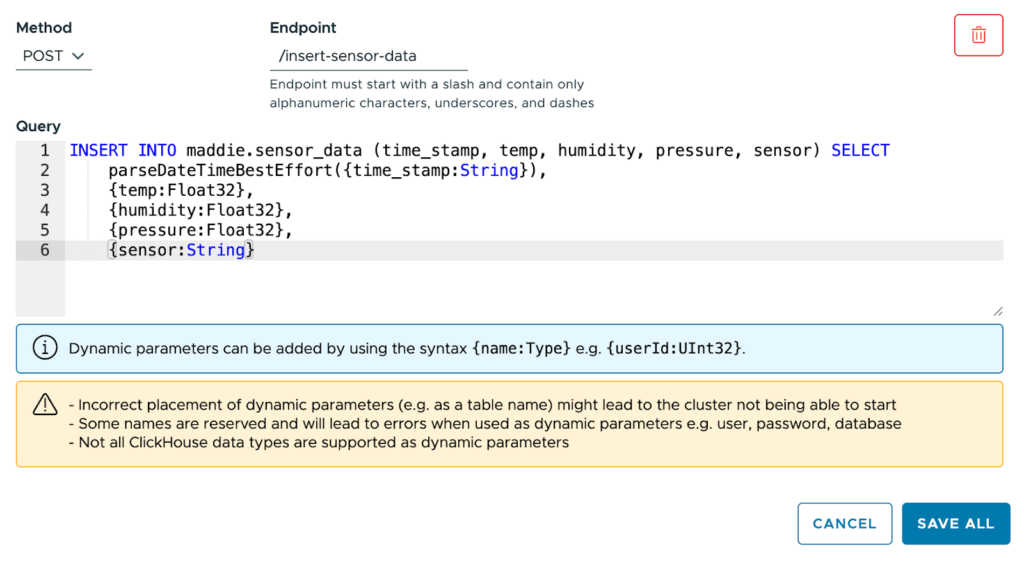
Figure 5. Defining a new ClickHouse endpoint
Select the POST method, name the endpoint /insert-sensor-data, and paste this statement into the text box:INSERT INTO maddie.sensor_data (time_stamp, temp, humidity, pressure, sensor) SELECT
parseDateTimeBestEffort({time_stamp:String}),
{temp:Float32},
{humidity:Float32},
{pressure:Float32},
{sensor:String}
Our INSERT statement has five parameters: time_stamp, temp, humidity, pressure, and sensor. The temp, humidity, and pressure parameters are all Float32; those values come directly from the sensor. The sensor parameter, a String, is the name we give to the sensor to distinguish it from other sensors.
Click SAVE ALL and you’ll have an endpoint:

Figure 6. The new endpoint is defined
You’ll see a message that lets you know that the API endpoint isn’t fully configured inside ClickHouse:
Figure 7. The endpoint isn’t ready
When the message disappears, you’re ready to go. The editor gives you entry fields for all of the parameters in the query. Here we can fill in five values and test the endpoint to make sure it works :

Figure 8. Testing the endpoint
Enter some test values and click the RUN button. If the post works, you’ll get nothing:

Figure 9. Empty result = success
It’s a POST, after all, so you shouldn’t get any results unless something goes wrong. And here we’re running the query as user admin; you can also run the query as another user. That’ll be useful when we talk about access control later.
You can go to the Query tab of the Cluster Explorer to make sure the new data is in the database:
SELECT * FROM maddie.sensor_data;
   ┌──────time_stamp─────────┬──temp─┬─humidity─┬─pressure─┬───sensor─────┐
1. │ 2026-02-10 03:02:51.000 │ 21.39 │     48.3 │   1013.5 │ warehouse-01 │
   └─────────────────────────┴───────┴──────────┴──────────┴──────────────┘
We’ve tested the endpoint from within the ACM; let’s also test it with curl. First of all, we need the URL of our ClickHouse cluster. There’s a Connection Details link in the ACM:

Figure 10. The Connection Details link
Clicking the link brings up this dialog:

Figure 11. The URL for our ClickHouse cluster
Based on this example, the URL is https://api-test.demo-cluster.altinity.cloud:8443/insert-sensor-data. (See the Cluster Connection Details documentation if you need more information.) To test your endpoints, substitute your cluster’s URL and your username and password to run this command:
curl -X POST \
"https://api-test.demo-cluster.altinity.cloud:8443/insert-sensor-data?time_stamp=2026-02-19%2012:30:45&temp=22.53&humidity=45.29&pressure=1013.25&sensor=curl-test" \
  -u "demouser:demopassword" \
  -H "Content-Length: 0"
If this works, you won’t get any response at all. As above, you can make sure it worked on the Query tab:
SELECT * FROM maddie.sensor_data WHERE sensor = 'curl-test'
   ┌─────────────time_stamp──┬──temp─┬─humidity─┬─pressure─┬─sensor────┐
1. │ 2026-02-19 12:30:45.000 │ 22.53 │    45.29 │  1013.25 │ curl-test │
   └─────────────────────────┴───────┴──────────┴──────────┴───────────┘
Moving on to the Hardware
Now we’ve set up our database, created our API endpoint, and we’ve made sure everything works. Let the fun begin! We’ll set up the Raspberry Pi next; skip ahead to the Raspberry Pi Pico section if that’s your hardware platform.
Setting Up the Raspberry Pi
You’ll need a power supply and a micro SD card, of course. Burn the card image in the Raspberry Pi imager:
- Select your device type, then use the recommended OS: Raspberry Pi OS (64-bit), which is a port of Debian Trixie.
- Create the user
demouserwith a password ofdemopassword. (Creating a user with that username and password on the ClickHouse cluster makes things simpler.) - Enter your SSID and password so the Pi connects to wifi automatically whenever it boots.
- Enable SSH with password authentication. This makes things easier, because we can use the Raspberry Pi without a keyboard, mouse, or monitor.
- There’s no need to enable Raspberry Pi Connect.
- With those options set, burn the image to the SD card.
Once your micro SD card is ready, insert it into your Raspberry Pi and power it up. When your RaspberryPi is up and running, SSH into it and update the system:sudo apt update
sudo apt upgrade -y
Next, configure the I2C interface:sudo raspi-config
Navigate through the menus:
- Select option 3: Interface Options → Enter
- Select option I5: I2C → Enter
- Would you like the ARM I2C interface to be enabled? → Select Yes → Enter
- Press Enter at the confirmation message
- Tab to Finish → Enter
Now restart the system:sudo reboot
When the system is back, install the Python tools and other things we’ll need to work with the I2C interface (they may be installed already, but this will make sure they are):sudo apt install -y python3-pip python3-venv git i2c-tools
Now we need to connect the sensor to the Raspberry Pi
Wiring Up the BME680
Wire the BME680 to the Raspberry Pi like this:

Figure 12. Pinouts for the Raspberry Pi and the BME680
The pinouts are (they’re the same for all Raspberry Pi models since at least 2014):
| BME680 pin | Raspberry Pi pin |
|---|---|
Power in (3.3V, NOT 5V) – labeled VCC on the generic board shown in Figure 12, labeled 2-6V on the Pimoroni breakout board, and labeled VIN on the Adafruit breakout board | 1 |
SDA or SDI | 3 |
SCL or SCK | 5 |
| Ground (you can use any of the Raspberry Pi’s eight ground pins, but pin 9 is the most convenient) | 9 |
NOTE: The Adafruit breakout board uses SPI terminology (SDI and SCK) instead of I2C. It also has pins labeled SDO and CS; leave those disconnected.
With the BME680 wired up, run i2cdetect -y 1 to make sure it’s detected by the system:i2cdetect -y 1
0 1 2 3 4 5 6 7 8 9 a b c d e f
00: -- -- -- -- -- -- -- –
10: -- -- -- -- -- -- -- -- -- -- -- -- -- -- -- –
20: -- -- -- -- -- -- -- -- -- -- -- -- -- -- -- –
30: -- -- -- -- -- -- -- -- -- -- -- -- -- -- -- –
40: -- -- -- -- -- -- -- -- -- -- -- -- -- -- -- –
50: -- -- -- -- -- -- -- -- -- -- -- -- -- -- -- –
60: -- -- -- -- -- -- -- -- -- -- -- -- -- -- -- –
70: -- -- -- -- -- -- 76 –
The BME680 should appear on slot 76 or 77. If all you see are double dashes (–),unwire the BME680 immediately. Especially if the BME680 is so hot you can barely touch it. (A moment of silence, please, for the sensor your author managed to wire up incorrectly. May it rest in peace.)
Installing the Code
To start, clone the example repo:git clone https://github.com/altinity/examples
Switch to the examples/bme680_clickhouse_demo/raspberry_pi directory. Set up the Python virtual environment and activate it: python -m venv venv
source venv/bin/activate
Once the environment is active, the command-line prompt should start with (venv):(venv) demouser@pizero-2w:~/examples/bme680_clickhouse_demo/raspberry_pi $
BTW, you can make sure you don’t have to call the source command again with this command:echo 'source ~/examples/bme680_clickhouse_demo/venv/bin/activate' >> ~/.bashrc
Next, make sure pip is up-to-date:pip install --upgrade pip
The requirements.txt file tells pip exactly what we need, so use it to set up our dependencies:pip install -r requirements.txt
Before we run the script that posts data to ClickHouse, run python test_bme680.py to make sure it’s actually working. Running python test_bme680.py writes the sensor data to the console every 3 seconds:Polling sensor (Ctrl+C to exit)
Temp: 27.57°C
Pressure: 1003.43 hPa
Humidity: 17.43%
------------------------------
Temp: 27.56°C
Pressure: 1003.42 hPa
Humidity: 17.43%
------------------------------
Temp: 27.55°C
Pressure: 1003.43 hPa
Humidity: 17.44%
------------------------------
^C
Exiting…
Type Ctrl+C to exit the script.
Configuring and Running the Code
At this point, the Raspberry Pi and the BME680 are working together. The script that reads the sensor and POSTs it to our ClickHouse endpoint is sensor_to_clickhouse.py. We need to configure it with our username, password, and the URL of our endpoint. First, copy .env.example to .env and set your username and password:# ClickHouse Credentials
# Copy this file to .env and fill in your actual credentials
CLICKHOUSE_USERNAME=your_username_here
CLICKHOUSE_PASSWORD=your_password_here
(Worry not, the repo contains a .gitignore file that makes sure you won’t accidentally commit the .env or config.json files.)
Now copy config.json.example to config.json and edit it to include your endpoint’s URL:{
"endpoint_url": "https://api-test.demo-cluster.altinity.cloud:8443/insert-sensor-data",
"sample_interval": 60,
"sensor_name": "warehouse-01",
"log_to_console": true,
"temp_adjustment": 0.0
}
Make sure endpoint_url ends with /insert-sensor-data, the name of the endpoint we defined in the ACM.
There are other parameters:
sample_interval– how many seconds between readingssensor_name– whatever you’d like to call this sensorlog_to_console– set to false if you don’t want to see console messages every time the script sends data to the endpointstemp_adjustment– lets you adjust the temperature reading by some number of degrees Celsius. Depending on how you have the sensor wired to the Raspberry Pi and what model of Raspberry Pi you’re using, heat from the Raspberry Pi may skew the temperature readings.
Everything is ready, so let’s run python sensor_to_clickhouse.py to start writing data to ClickHouse:
Sensor Logger initialized successfully!
Endpoint: https://api-test.demo-cluster.altinity.cloud:8443/insert-sensor-data
Sample interval: 60 seconds
Sensor: warehouse-01
Temperature offset: 0.0
Starting sensor data collection...
Press Ctrl+C to stop

✓ Data sent successfully at 2026-02-20 15:10:11
  Temp: 25.19°C (raw: 25.19°C), Humidity: 30.01%, Pressure: 990.13 hPa
✓ Data sent successfully at 2026-02-20 15:11:17
  Temp: 25.21°C (raw: 25.21°C), Humidity: 30.0%, Pressure: 990.13 hPa
^C

Stopping sensor logger...
Goodbye!
Hurrah! We’ve successfully configured the hardware and software we need to write data to ClickHouse through our API endpoint. There are some things we should do to keep everything secure, however. You can skip past the Raspberry Pi Pico section for the details.
Setting Up the Raspberry Pi Pico
You’ll need a micro USB cable to connect the Pico to your PC. To start, we need to flash the MicroPython runtime to the Pico. Insert the micro USB cable into the Pico, hold down the Pico’s BOOTSEL button, then plug the other end of the cable into your machine. The Pico will show up on your desktop as a new USB flash drive:

Figure 13. The Pico shows up as a flash drive
Go to the MicroPython Pico W site and download the latest version of the .uf2 file for the Pico W. Copy that file to the flash drive that represents the Pico. When that file is copied, the Pico will install MicroPython and reboot. The Pico is now initialized, so we’re ready to wire up the sensor.
Wiring Up the BME680
Put the Pico and the sensor breakout board on a breadboard and wire them up like this:

Figure 14. Pinouts for the Raspberry Pi Pico and the BME680
NOTE: The pinouts on the Raspberry Pi Pico are numbered differently from Linux-based Raspberry Pis. Here’s how the pins are numbered:
| Raspberry Pi Pico | Raspberry Pi |
|---|---|
1 40etc. | 1 2etc. |
With that in mind, wire up the BME680 as shown in Figure 13 above:
| BME680 pin | Raspberry Pi Pico pin |
|---|---|
SDA or SDI | 1 |
SCL or SCK | 2 |
| Ground | 33 |
Power in (3.3V, NOT 5V) – labeled VCC on the generic board shown in Figure 13, 2-6V on the Pimoroni breakout board, and VIN on the Adafruit breakout board | 36 |
NOTE: The Adafruit breakout board uses SPI terminology (SDI and SCK) instead of I2C. It also has pins labeled SDO and CS; leave those disconnected.
Now it’s time to get the code running on the Pico.
Installing the Code
To start, clone the example repo:git clone https://github.com/altinity/examples
Switch to the examples/bme680_clickhouse_demo/raspberry_pi_pico directory.
There are a couple of ways to install the code on the Pico; here we’ll focus on Thonny, an IDE that works with microcontrollers. (There are other ways to copy files; see the raspberry_pi_pico/SETUP.md file for the details.) When you install it, you’ll see something like this:
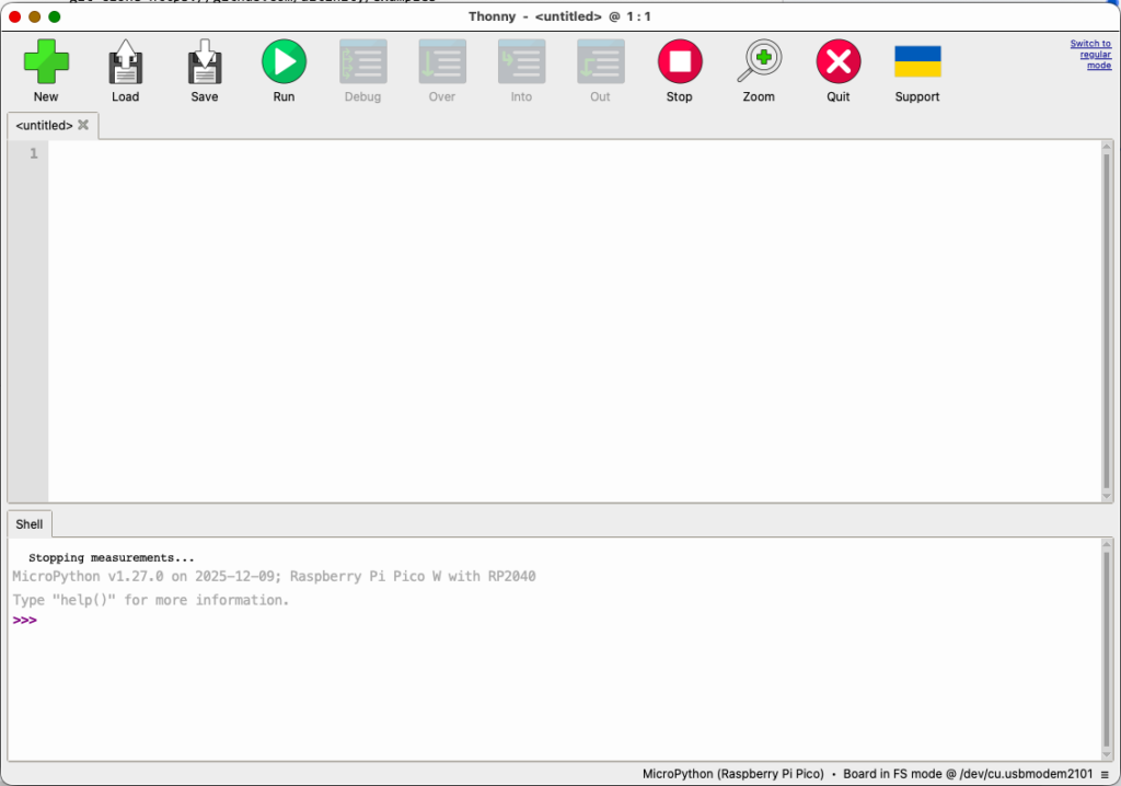
Figure 15. The Thonny IDE
Click the list of devices in the lower right corner of the window and select the Pico:

Figure 16. Connecting to the Pico
Click the View → Files menu item to open the Files tab. Navigate to the examples/bme680_clickhouse_demo/raspberry_pi_pico directory. Right-click on the file main.py, then choose Upload to /:

Figure 17. Uploading the code to the Pico
The Python script uses the bme680.py module. Download the latest version of bme680.py from the BME680-Micropython repo onto your machine, then use the same process to copy it to the Pico. The script and the BME680 library should be on the Pico:

Figure 18. The main script and the sensor library are on the Pico
Configuring and Running the Code
The main script tries to load your configuration details from a file named config.py. (The project’s .gitignore file ensures that your config.py file will never be committed.) Double-click on the config.example.py file in the Raspberry Pi Pico section of the Files tab. That will open the sample configuration file in the IDE:

Figure 19. The sample configuration file
We need to save a copy of this file as config.py. Click the File → Save As… menu. You’ll be asked where you want to save the file:

Figure 20. Thonny asks where you want to save the file
Click Raspberry Pi Pico, then save the file as config.py:

Figure 21. Saving the sample configuration file on the Pico
Edit config.py and enter the correct parameters for your environment:
# ============ CONFIGURATION ============
WIFI_SSID = "Wu-TangLAN"
WIFI_PASSWORD = "7thChamber"
CLICKHOUSE_URL = "https://example-cluster.altinity.cloud:8443/insert-sensor-data"
CLICKHOUSE_USER = "demouser"
CLICKHOUSE_PASSWORD = "demopassword"
SENSOR_NAME = "warehouse-01"
POST_INTERVAL = 60  # seconds between readings
When you’ve configured them correctly, click the Save button. Now double-click main.py in the Raspberry Pi Pico section of the files tab. Click Run. You can watch the action in the Shell tab:

Figure 22. The Pico successfully initializing and writing data to ClickHouse
Figure 22 is nothing but good news! The script found the BME680, connected to wifi, set the system time, then posted a reading to ClickHouse. (Without setting the system time, the Pico defaults to January 1, 2021.) Thonny makes it easy to get the code on the Pico, and you have a console that lets you diagnose any problems. Once the code is working, you can disconnect the Pico from your machine. There’s no need to connect the Pico to your machine again; anytime it’s powered up, the Pico finds main.py and runs it. Figure 23 shows the Pico running on battery power, with no other computer in sight:

Figure 23. The Pico running on battery power
Access Control for Your Endpoint
It’s great that everything is working, but you definitely want tight control on who can insert data into your database. There are a couple of things you should do to keep your data safe.
Define Allowed IP Addresses
The ACM lets you define a list of allowed IP addresses for your cluster. With those addresses defined, any request that comes from any other IP address will be ignored. Put the IP addresses of your authorized users on the list, and your endpoint is much more secure.
Create User Accounts with Limited Access
You can only access the endpoints with valid credentials. You should create user accounts with limited access. The ACM makes it easy to manage your user accounts, and you can restrict the access of those accounts to only the databases you specify. And as we mentioned earlier, you can test the endpoints in the endpoint editor by running a query as a particular user.
As Usual, Thanks to Claude!
See the raspberry_pi/AGENTS.md and raspberry_pi_pico/AGENTS.md files for complete details on your author’s interactions with Claude as they worked out the details of the code, hardware configuration, and other details. (Things got a little spicy at times.)
Summary
ClickHouse’s API endpoints simplify the code that goes into the applications that work with ClickHouse data, hiding the structure of your database in the process. The Altinity Cloud Manager makes it easy to create, test, and manage endpoints, as well as manage users and control what they can access. In this post, we’ve seen how to use API endpoints to allow very small, lightweight devices to create records in a ClickHouse database. It’s a powerful, elegant way to collect data that can be analyzed in real time.
If you have questions, please contact us at Altinity or join the discussion on our Slack channel. And please sign up for a free trial Altinity.Cloud account and try it out for yourself!
Appendix A: Parts List
We ran the code on these machines:
There are several breakout boards for the BME680:
- Pimoroni BME680, in a package that includes a right-angle female header as shown in Figures 1 and 2 above
- Adafruit BME680
- hiBCTR Environmental Sensor Module, one of many generic boards
All of these sensors use the Bosch BME680 chip, and there are many form factors and vendors to choose from. We really like the combination of the Pimoroni and the right-angled female header. The pinouts match the RaspberryPi perfectly, letting you attach the sensor without jumper wires.
For the battery-powered Pico setup, we added:
- Adafruit Lithium Ion Polymer battery (3.7V, 2500mAh)
- Adafruit PowerBoost 500 charger
Starting with a fully charged battery, the Pico ran for roughly 38 hours.
NOTE: All of these items can be purchased from multiple sources around the web. Look for the combination of price, availability, and shipping costs that work for you. No one at Altinity (including your author) has any commission plan or partnership with any of these vendors; we’re just passing along what we used in building this sample.
Appendix B: Urge Overkill
Nvidia’s Jetson Nano is a Linux-based SBC with a 128-core NVIDIA Maxwell GPU. That’s overkill for running a small Python script that reads a sensor, but it works. (Your author was obsessed with getting this code to work on every SBC around the house.) The pinouts we need for the Nano are the same as those for the Raspberry Pis; wire the BME680 as we discussed in the Raspberry Pi section above. If you’ve got the Pimoroni breakout board, it simply plugs in:

Figure 24. A Jetson Nano with a BME680 sensor attached
With a couple of minor exceptions, the instructions for getting the example running on the Jetson Nano are the same as for the Raspberry Pi. However, the machine runs on Ubuntu 18.04 (yes, an eight-year-old OS), so the more recent versions of the packages used by the Raspberry Pi aren’t available. To compensate, the raspberry_pi/jetson-requirements.txt file specifies older versions of the packages. Use it instead of the requirements.txt file:
pip install -r jetson-requirements.txt
You may need to use the python3 command instead of python as you follow the Raspberry Pi steps above, and you’ll need to run i2cdetect -y -r -a 1 to check the connection to the BME680. Beyond that, the Jetson Nano should work just fine. It should also work with the Jetson Orin Nano. Buying another SBC and testing it is left as an exercise for the reader. If you try it, let us know how it goes!
The post Using Altinity.Cloud to Log Sensor Data with ClickHouse® Endpoints appeared first on Altinity | Run open source ClickHouse® better.
]]>The post Project Antalya 2026 Roadmap appeared first on Altinity | Run open source ClickHouse® better.
]]>Project Antalya was started internally a year ago, and was first announced to the community in April 2025. We wanted to solve the problem of high storage cost for big data sets, and add compute-storage separation for users of open source ClickHouse®. Project Antalya is based on three simple ideas: Parquet on object storage as an open data format, Iceberg as an open table format, and compute swarms as an open execution model. We have been implementing those ideas in ClickHouse throughout 2025. What comes next in 2026?
Iceberg as a first-class citizen in ClickHouse
During 2025 Iceberg became the de-facto standard for data lakes. There are strong reasons for that. Iceberg provides a true universal interface to tables on object storage. It also has a transaction model that allows it to be used as a storage layer for DBMS. And it is open, supported by hundreds of products and libraries.
While there was a lot of progress integrating Iceberg into ClickHouse in 2025, it is still far from perfection. Our goal is to make Iceberg tables as easy to use as MergeTree, for storing and querying data. In particular, we want the full CREATE TABLE functionality that would support partitioning, sorting, schema inference from a source table, and table settings. Other DDL commands are needed as well, such as DROP TABLE, TRUNCATE TABLE, and ALTER TABLE. The latter one is especially intriguing to implement and test.
The same is true for writing into Iceberg tables. While the basic functionality was added into ClickHouse in Q3-Q4/2025, it still lacks the convenience of MergeTree tables. Full support should come in the following months.
Swarming around Data
Compute Swarms are among the best features of Project Antalya, and the most successful so far. Swarm nodes do not keep any data and schema, and therefore can be almost instantly launched and used to query Parquet data from Iceberg tables or object storage directly. We put a lot of effort into proper cache tuning and job distribution, and proved that ClickHouse with Antalya Swarm extension can outperform MergeTree containing the same data.
While the swarm computational model is extremely powerful, we want to make it even better. In particular, we plan to introduce native support for Standalone Swarms that can be used from any ClickHouse instance, not just Antalya builds. Other planned features include better support for joins.
The bigger story is an extension of swarm computing model outside of query only. We plan to add features that would make it easy to use swarms for data transformations like inserting new data and compaction of Parquet files. These operations typically required heavy weight Spark jobs in the past, but with compute swarms it will be much easier and faster.
Tiered Storage and Hybrid Tables
When we started Antalya we wanted to solve a problem for our users that sounded trivial: how to store a lot of data in the cloud in the most efficient way without sacrificing legendary ClickHouse performance. This problem is not easy to solve. Project Antalya approaches it by using Iceberg as a cold tier for ClickHouse MergeTree data. We have made two major additions to ClickHouse for that. ALTER TABLE EXPORT PART and EXPORT PARTITION allow exporting data from MergeTree to Iceberg. Hybrid Tables provide an interface to query from MergeTree and Iceberg tiers as from a single table.
We are continuing to invest in improvements in both features to ensure that they can operate at scale, and support transparent, transactional movement of data between MergeTree and Iceberg. We’re shooting to have this complete by Q3 2026.
Performance, Security and Other Features
Project Antalya gained a lot of interest from ClickHouse users and community. Engineers started to try it out for various use cases and discover new applications. That generated user requests that we always take seriously. One example from 2025 is how Antalya Compute Swarms can be used as a query engine for new AWS service S3 Table buckets.
We plan more features like this. We have already tested support for Snowflake Polaris. Next step is to extend Antalya to use Google Metastore, Unity, and other popular catalogs. There are very few efficient execution engines for data lakes. Data is often abandoned because there is no easy way to query it. ClickHouse query speed and scalability of Antalya swarms will convert such data swamps to data jets!
Another important focus is security. The security model for data lakes is very convoluted. We need to support OAuth for accessing catalogs and respect security models configured via catalogs. ClickHouse RBAC and row-level access policies allow fine grain access control to sensitive data. We plan to apply this efficiently to Iceberg as well.
Project Antalya Full Throttle
2025 was the incubation year for Project Antalya. It proved that all three ideas – Parquet, Iceberg and Swarms – are feasible technologies to deliver a capable real-time data lake engine. In 2026, Antalya builds will mature into a production grade technology suitable for a wide range of use cases. The data sizes are growing, and Project Antalya is the right technology to keep up with this growth.
Project Antalya is an open source project based on ClickHouse that everybody can use and contribute back. We do not develop it just for ourselves. We believe that open source, open storage and and an open query execution model is the desired foundation for every user. When it is open – there is no vendor lock-in.
The more detailed Project Antalya 2026 roadmap is publicly available. If you know C++ and want to develop some cool stuff – give us a all. We welcome contributions and new community members. Join us!
The post Project Antalya 2026 Roadmap appeared first on Altinity | Run open source ClickHouse® better.
]]>The post Five Ways to Make Your ClickHouse® Slow (and How to Avoid Them) appeared first on Altinity | Run open source ClickHouse® better.
]]>Presenters: Robert Hodges
We all want analytics that deliver real-time results, and ClickHouse is legendary for speed. New users are therefore surprised when their first big ClickHouse deployment runs like a slug.
This talk reveals the biggest performance killers, including poor input batching, flawed schemas, bad queries, insufficient indexing, and skimping on resources.
We’ll explain exactly how each slows you down and how to avoid them. You’ll quickly get your system back to gazelle-like speed.
Here are the slides:
The post Five Ways to Make Your ClickHouse® Slow (and How to Avoid Them) appeared first on Altinity | Run open source ClickHouse® better.
]]>The post Deploying Single-Node ClickHouse® on Small Servers appeared first on Altinity | Run open source ClickHouse® better.
]]>The truth is, ClickHouse’s raw performance is so impressive that a single well-configured server can handle workloads that would bring traditional databases to their knees. For development environments, staging setups, or even low-to-moderate traffic production systems, a single node deployment makes a lot of sense. You get all the analytical power without the operational complexity of managing a cluster.
Recommended Hardware
ClickHouse is not lightweight, but it can be tuned to run on minimal hardware: 4+ CPU cores, 8GB+ RAM, SSD storage.
The minimum viable setup is around 4GB RAM, but you’ll want at least 8GB for any real workload.
Installing ClickHouse
There are many ways to install ClickHouse. There is this one-liner from the official documentation:
curl https://clickhouse.com/ | shWarning: Installing with this command will install the latest commit from `main`, and will create some configuration files on your system. We don’t recommend using this command.
Instead, you can use Docker and the official ClickHouse Docker images or the Altinity Stable Builds to run a containerized version of ClickHouse.
In my own home lab, I’m using NixOS’s built-in support for OCI containers to run a containerized ClickHouse as a systemd service.
Understanding ClickHouse’s Configuration Structure
However you’ve got ClickHouse installed, let’s review the configuration files. The server ships with two main files:
- /etc/clickhouse-server/config.xml — Server settings
- /etc/clickhouse-server/users.xml — User profiles and access controls
Important: you should never modify these files directly. ClickHouse is designed to load additional configuration from subdirectories, which means you can override any setting without touching the vendor files. This makes upgrades painless and your customizations easy to track.
The directory structure looks like this:
/etc/clickhouse-server/
├── config.xml           # Don't modify
├── users.xml            # Don't modify
├── config.d/            # Your server config overrides
│   ├── listen.xml
│   ├── memory.xml
│   └── storage.xml
└── users.d/             # Your user/profile overrides
    └── profiles.xml
Files in config.d/ and users.d/ are processed alphabetically and merged with the base configuration. This pattern is common in Unix-style configuration, and ClickHouse implements it well.
Basic Configuration: Listening on All Interfaces
Out of the box, ClickHouse only listens on localhost. That’s secure by default, but not useful if you need to connect from other machines. The first configuration file we’ll create enables network access:
<!-- /etc/clickhouse-server/config.d/listen.xml -->
<clickhouse>
    <listen_host>0.0.0.0</listen_host>
</clickhouse>
This tells ClickHouse to accept connections on all network interfaces. A few important notes:
- Security matters: Once you bind to 0.0.0.0, anyone who can reach your server can attempt to connect. Make sure you have firewall rules in place, and consider setting up authentication (covered in the official docs).
- IPv6: If you need IPv6, add <listen_host>::</listen_host> as well.
Create this file and restart ClickHouse (assuming you’re using systemd):
sudo systemctl restart clickhouse-serverVerify it’s listening:
curl http://localhost:8123/
# Should return "Ok."
(You should also be able to do this from a remote host, replacing `localhost` with the IP address of the host where ClickHouse is running.)
Memory Configuration: Standard vs Constrained Environments
Memory management is where ClickHouse configuration gets interesting. The defaults assume you’re running on a beefy server with plenty of RAM, but not everyone has that luxury.
Standard Configuration (16GB+ RAM)
If you have a server with 16GB or more of RAM, the defaults are reasonable. You might still want to set explicit limits to prevent runaway queries from consuming everything:
<!-- /etc/clickhouse-server/config.d/memory.xml -->
<clickhouse>
    <!-- Cap server memory at 12GB, leaving headroom for the OS -->
    <max_server_memory_usage>12884901888</max_server_memory_usage>
</clickhouse>
This is a “set it and forget it” configuration. ClickHouse will respect these limits and throw errors rather than letting the OOM killer terminate your process.
Constrained Configuration (4-8GB RAM)
Running ClickHouse on a smaller server requires more aggressive tuning. When I first set up ClickHouse on an 8GB VM, I hit out-of-memory errors within hours. The problem wasn’t query execution—it was background merge operations consuming all available memory.
The official documentation contains a guide on which settings to adjust for low memory environments.
Disabling System Logs
ClickHouse maintains numerous internal log tables for debugging and monitoring. These are invaluable for troubleshooting, but they also consume memory, disk space, and CPU cycles. For resource-constrained deployments or high-volume systems, you can selectively disable them:
<!-- /etc/clickhouse-server/config.d/disable_logs.xml -->
<clickhouse>
    <!-- Disable system logs to save resources -->
    <trace_log remove="1"/>
    <text_log remove="1"/>
    <metric_log remove="1"/>
    <asynchronous_metric_log remove="1"/>
    <query_log remove="1"/>
    <part_log remove="1"/>
    <processors_profile_log remove="1"/>
    <query_views_log remove="1"/>
    <query_metric_log remove="1"/>
</clickhouse>
The remove=”1″ attribute completely disables each log table.
NB: Think carefully before disabling query_log. It’s your primary tool for understanding what queries are running and how long they take. In production, I’d recommend keeping it enabled and instead setting a short TTL to limit disk usage:
<query_log>
    <database>system</database>
    <table>query_log</table>
    <flush_interval_milliseconds>7500</flush_interval_milliseconds>
    <ttl>event_date + INTERVAL 7 DAY DELETE</ttl>
</query_log>
Storage Configuration
Storage policies control how ClickHouse manages disk space. At minimum, you should configure free space thresholds to prevent your disk from filling completely:
<!-- /etc/clickhouse-server/config.d/storage.xml -->
<clickhouse>
    <storage_configuration>
        <disks>
            <default>
                <!-- Always keep 2GB free on disk -->
                <keep_free_space_bytes>2147483648</keep_free_space_bytes>
            </default>
        </disks>
        <policies>
            <default>
                <volumes>
                    <main>
                        <disk>default</disk>
                        <!-- Cap individual part sizes at 10GB -->
                        <max_data_part_size_bytes>10737418240</max_data_part_size_bytes>
                    </main>
                </volumes>
            </default>
        </policies>
    </storage_configuration>
</clickhouse>
The keep_free_space_bytes setting is critical—ClickHouse will stop accepting writes rather than fill your disk. The max_data_part_size_bytes limit prevents any single data part from growing too large.
MergeTree Engine Settings
The MergeTree family of engines is the heart of ClickHouse. These global settings affect all MergeTree tables:
<!-- /etc/clickhouse-server/config.d/merge_tree.xml -->
<clickhouse>
    <merge_tree>
        <!-- Pool entry thresholds -->
        <!-- These must be less than: background_pool_size * background_merges_mutations_concurrency_ratio -->
        <!-- With pool_size=4 and ratio=2, max is 8, so we use 6 -->
        <number_of_free_entries_in_pool_to_execute_mutation>6</number_of_free_entries_in_pool_to_execute_mutation>
        <number_of_free_entries_in_pool_to_execute_optimize_entire_partition>6</number_of_free_entries_in_pool_to_execute_optimize_entire_partition>
        <number_of_free_entries_in_pool_to_lower_max_size_of_merge>6</number_of_free_entries_in_pool_to_lower_max_size_of_merge>
        <!-- Parts thresholds - increase to prevent "Too many parts" errors -->
        <parts_to_throw_insert>1500</parts_to_throw_insert>
        <parts_to_delay_insert>750</parts_to_delay_insert>
        <!-- Use compact format for small parts to reduce memory footprint -->
        <min_bytes_for_wide_part>10485760</min_bytes_for_wide_part>
        <min_rows_for_wide_part>100000</min_rows_for_wide_part>
    </merge_tree>
</clickhouse>
A few key points:
“Too many parts” errors: ClickHouse has built-in protection against accumulating too many unmerged parts. If merges can’t keep up with inserts, you’ll get errors. The parts_to_throw_insert and parts_to_delay_insert settings control these thresholds. Increasing them gives merges more time to catch up, but very high values can lead to performance degradation during queries.
Wide vs compact part format: ClickHouse stores data parts in two formats. Wide format is faster for queries but uses more memory. Compact format is more memory-efficient for small parts. The min_bytes_for_wide_part and min_rows_for_wide_part settings control the threshold. On memory-constrained systems, keeping these values high ensures small parts stay in compact format.
Pool entry settings: These control when certain operations are allowed to run based on how many background threads are available. The values must be less than background_pool_size * background_merges_mutations_concurrency_ratio. If you set background_pool_size to 4 and the ratio to 2, that gives you 8 total slots—so these values should be below 8.
Verifying Your Configuration
After creating your configuration files and restarting ClickHouse, verify everything is working:
# Check ClickHouse is listening on HTTP port
curl http://localhost:8123/

# Connect via native client
clickhouse-client --query "SELECT 1"

# View applied memory settings
clickhouse-client --query "SELECT name, value FROM system.settings WHERE name LIKE '%memory%' ORDER BY name"

# Check current memory usage
clickhouse-client --query "SELECT metric, value FROM system.asynchronous_metrics WHERE metric LIKE '%Memory%'"

# Verify MergeTree settings
clickhouse-client --query "SELECT name, value FROM system.merge_tree_settings WHERE name LIKE '%parts%'"
If something isn’t applied correctly, check the server logs:
sudo journalctl -u clickhouse-server -fClickHouse logs configuration errors at startup, including which files were loaded and any parsing issues.
Conclusion and Next Steps
You now have a stable development-ready single-node ClickHouse deployment with:
- Network accessibility for remote connections
- Memory limits appropriate for your hardware
- Optimized merge settings to prevent OOM conditions
- Storage policies to protect disk space
- Query-level resource limits
This configuration will handle most single-node workloads without surprises. As your data grows, monitor these metrics:
- system.parts table for part counts (watch for “Too many parts” warnings)
- system.asynchronous_metrics for memory pressure
- system.query_log for slow queries (if you kept it enabled)
When a single node is no longer enough, ClickHouse’s clustering capabilities scale horizontally. But don’t rush to add complexity—you might be surprised how much a single well-configured server can handle.
Further Reading
- Altinity Knowledge Base — Excellent resource for ClickHouse operations
- ClickHouse Documentation — Official reference
- Configure ClickHouse for Low Memory Environments — Deep dive on memory tuning
- Server Config Files — Configuration structure details
- Tracing ClickHouse with OpenTelemetry — Native OpenTelemetry support
The post Deploying Single-Node ClickHouse® on Small Servers appeared first on Altinity | Run open source ClickHouse® better.
]]>The post Live-coding with MooseStack: Let’s ship real-time dashboards and AI chat powered by ClickHouse® appeared first on Altinity | Run open source ClickHouse® better.
]]>Presenters: Joshua Lee & Chris Crane
What if you could build a custom AI-powered chat interface into your application – powered by ClickHouse and Kafka for real-time answers – in under an hour?
Watch us for this live-coding session, where we’ll combine open-source tools to showcase a demo application fed by the Bluesky firehose.
You’ll learn how to build, deploy, and operate ClickHouse-powered real-time user experiences in your existing application stack with your Python / Typescript application framework of choice.
We’ll get hands-on with data pipelines, workflows, MCPs, and APIs, all backed by the performance of ClickHouse. We’ll explore coding locally in the IDE with a local dev server, and shipping into production with Altinity Cloud and Fiveonefour.
Come for a technical deep dive that will culminate in us live-coding an AI-chat assistant into the demo application.
Here are the slides:
The post Live-coding with MooseStack: Let’s ship real-time dashboards and AI chat powered by ClickHouse® appeared first on Altinity | Run open source ClickHouse® better.
]]>