
Luckily, we have a tradition at work , whenever something security-related comes up, we just ping Amnjeet
He showed me how it works , and I have to say, I loved it. It’s refreshingly simple.
You can download the notebook here:
You just select a folder in your Lakehouse and turn it on.
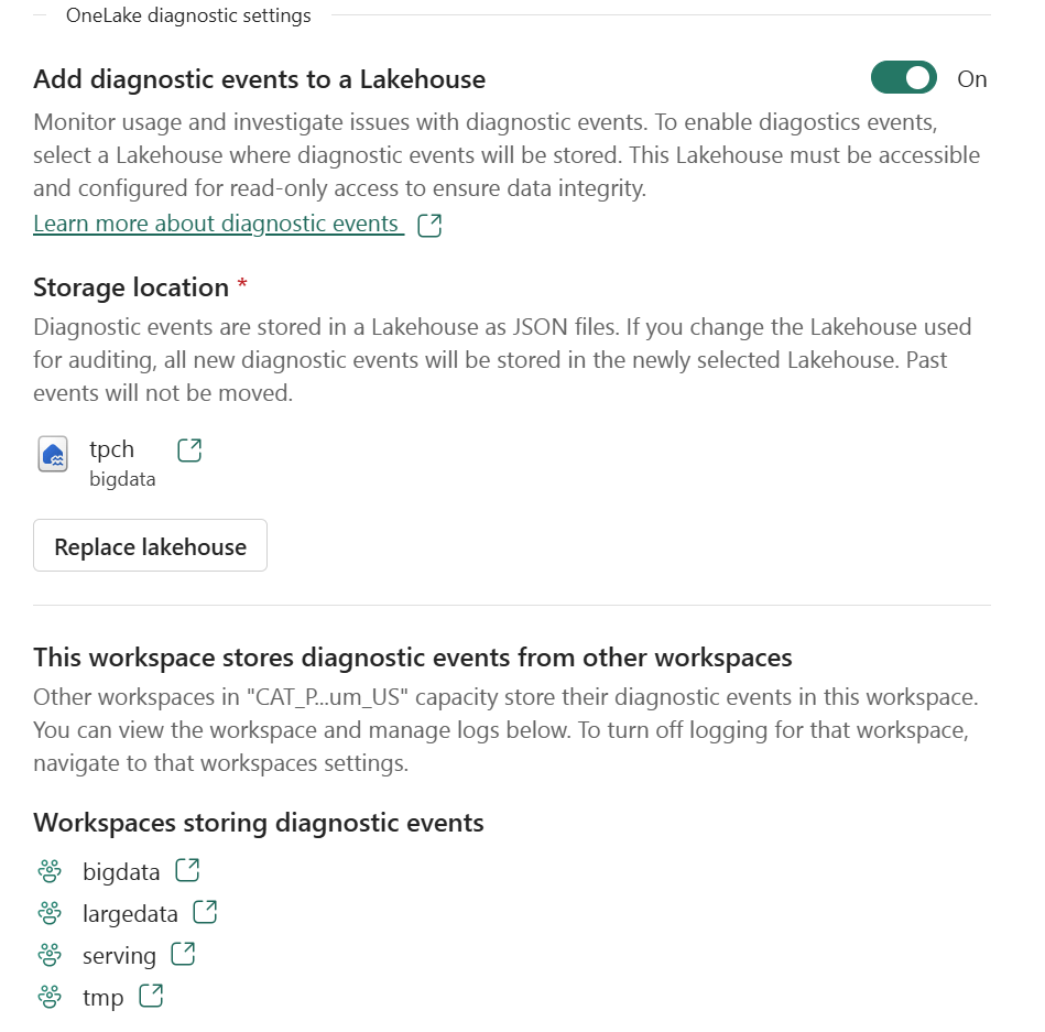
That’s it , the system automatically starts generating JSON files, neatly organized using Hive-style partitions, By default, user identity and IP tracking are turned off unless an admin explicitly enables them. You can find more details about the schema and setup here.
What the Logs Look Like
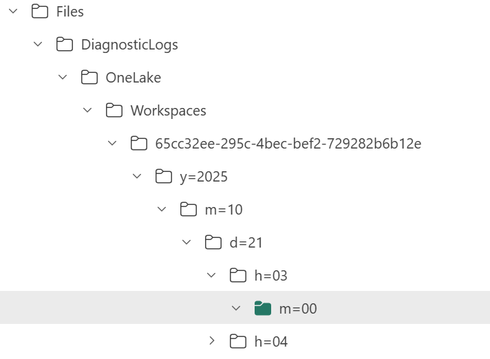
Currently, the logs are aggregated at the hourly level, but the folder structure also includes a partition for minutes (even though they’re all grouped at 00 right now).
Parsing the JSON Logs
Once the logs were available, I wanted to do some quick analysis , not necessarily about security, just exploring what’s inside.
There are probably half a dozen ways to do this in Fabric ; Shortcut Transform, RTI, Dataflow Gen2, DWH, Spark, and probably some AI tools too, Honestly, that’s a good problem to have.
But since I like Python notebooks and the data is relatively small, I went with DuckDB (as usual), but Instead of using plain DuckDB and delta_rs to store the results, I used my little helper library, duckrun, to make things simpler ( Self Promotion alert).
Then I asked Copilot to generate a bit of code for registering existing functions to look up the workspace name and lakehouse name from their GUIDs in DuckDB, using SQL to call python is cool
The data is stored incrementally, using the file path as a key , so you end up with something like this:
import duckrun

con = duckrun.connect('bigdata/tpch.lakehouse/dbo')

onelake_logs_path = (
    'abfss://[email protected]/'
    'tpch.Lakehouse/Files/DiagnosticLogs/OneLake/Workspaces/*/'
    'y=*/m=*/d=*/h=*/m=*/*.json'
)
Then I added only the new logs with this SQL script:
try:
    con.sql(f"""
        CREATE VIEW IF NOT EXISTS logs(file) AS SELECT 'dummy';
        SET VARIABLE list_of_files =
        (
            WITH new_files AS (
                SELECT file
                FROM glob('{onelake_logs_path}')
                WHERE file NOT IN (SELECT DISTINCT file FROM logs)
                ORDER BY file
            )
            SELECT list(file) FROM new_files
        );
        SELECT * EXCLUDE(data), data.*, filename AS file
        FROM read_json_auto(
            GETVARIABLE('list_of_files'),
            hive_partitioning = true,
            union_by_name = 1,
            FILENAME = 1
        )
    """).write.mode("append").option("mergeSchema", "true").saveAsTable('logs')
except Exception as e:
    print(f"An error occurred: {e}")
1- Using glob() to collect file names means you don’t open any files unnecessarily , a small but nice performance win.
2- DuckDB expand the struct using this expression data.*
3- union_by_name = 1 in case the json has different schemas
4- option(“mergeSchema”, “true”) for schema evolution in Delta table
Exploring the Data
Once the logs are in a Delta table, you can query them like any denormalize table.
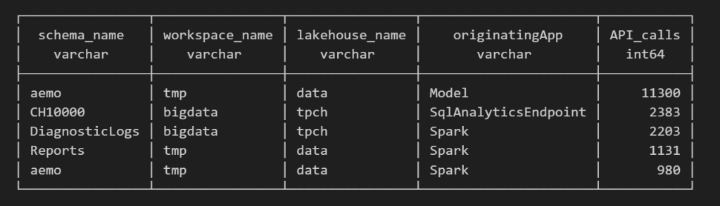
For example, here’s a simple query showing API calls per engine:
Note : using AI to get working regex is maybe the best thing ever
SELECT
    regexp_extract(resource, '([^&/]+)/([^&/]+)/(Tables|Files)(?:/([^&/]+))?(?:/([^&/]+))?', 4) AS schema_name,
    get_workspace_name(workspaceid) AS workspace_name,
    get_lakehouse_name(workspaceid, itemId) AS lakehouse_name,
    originatingApp,
    COUNT(*) AS API_calls
FROM logs
GROUP BY ALL
ORDER BY API_calls DESC
LIMIT 5;
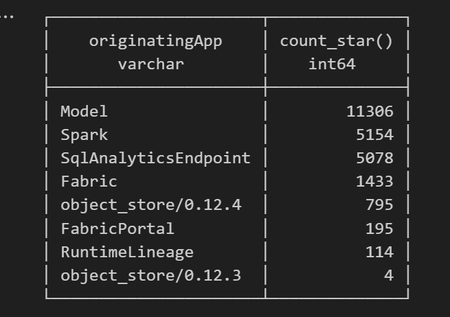
Fun fact: OneLake tags Python notebook as Spark.
Also, I didn’t realize Lineage calls OneLake too!
as I have already register Python functions as UDFs, which is how I pulled in the workspace and lakehouse names in the query above.
Takeaway
This was just a bit of tinkering, but I’m really impressed with how easy OneLake Diagnostics is to set up and use.
I still remember the horrors of trying to connect Dataflow Gen1 to Azure Storage ,that was genuinely painful (and I never even got access from IT anyway).
It’s great to see how Microsoft Fabric is simplifying these scenarios. Not everything can always be easy, but making the first steps easy really gives the feature a very good impression.
]]>In short: there is now a defined way to store GIS data in Parquet. Both Delta Lake and Apache Iceberg have adopted the standard ( at least the spec). The challenge is that actual implementation across engines and libraries is uneven.
- Iceberg: no geometry support yet in Java nor Python, see spec
- Delta: it’s unclear if it’s supported in the open source implementation (I need to try sedona and report back), nothing in the spec though ?
- DuckDB: recently added support ( you need nightly build or wait for 1.4)
- PyArrow: has included support for a few months, just use the latest release
- Arrow rust : no support, it means, no delta python support

The important point is that agreeing on a specification does not guarantee broad implementation. and even if there is a standard spec, that does not means the initial implementation will be open source, it is hard to believe we still have this situation in 2025 !!!
Let’s run it in Python Notebook
To test things out, I built a Python notebook that downloads public geospatial data, merges it with population data, writes it to Parquet, and renders a map using GeoPandas, male sure to install the latest version of duckdb, pyarrow and geopandas
!pip install -q duckdb  --pre --upgrade
!pip install -q pyarrow --upgrade
!pip install geopandas  --upgrade
import sys
sys.exit(0)
At first glance, that may not seem groundbreaking. After all, the same visualization could be done with GeoJSON. The real advantage comes from how geometry types in Parquet store bounding box coordinates. With this metadata, spatial filters can be applied directly during reads, avoiding the need to scan entire datasets.
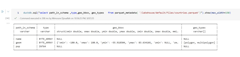
That capability is what makes the feature truly valuable: efficient filtering and querying at scale, note that currently duckdb does not support pushing those filters, probably you need to wait to early 2026 ( it is hard to believe 2025 is nearly gone)
 Workaround if your favorite Engine don’t support it .
A practical workaround is to read the Parquet file with DuckDB (or any library that supports geometry types) and export the geometry column back as WKT text. This allows Fabric to handle the data, albeit without the benefits of native geometry support, For example PowerBI can read WKT just fine
duckdb.sql("select geom, ST_AsText(geom) as wkt from '/lakehouse/default/Files/countries.parquet' ")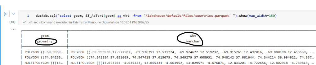
For PowerBI support to wkt, I have written some blogs before, some people may argue that you need a specialized tool for Spatial, Personally I think BI tools are the natural place to display maps data
The dataset I used contains the last seven years of Australian electricity market data. Although it’s public, the government agency only keeps archives for two months. I had saved the data during a previous job and kept it around as a hobby. It’s a great real-world workload with realistic data distribution. The CSV files are messy. Technically, they’re more like reports, with different sections stacked on top of each other and varying numbers of columns. That’s often what you encounter in real projects, not the neat, well-structured datasets you see in demos.
For example, being able to read a CSV file with a variable number of columns is a critical feature. Yet this rarely gets mentioned in synthetic benchmarks.
To create a clean environment for testing, I copied the data from one Lakehouse in onelake to a brand-new workspace. I could have used a shortcut, but I wanted to start from scratch. The binary copy took just 2 minutes, with no transformations, which gives a throughput of 1.4 GB per second. That’s pretty good for a 150 GB uncompressed dataset.

The default configuration for Fabric Python notebooks includes 2 cores and 16 GB of RAM. That’s roughly the same size as Google Colab. But you can easily increase the number of cores to 4, 8, 16, 32, or even 64. At 64 cores, you get nearly half a terabyte of RAM. That’s a serious machine.
The job itself is simple. Ingest and process the data using several Python engines, then save the result as a Delta table. The raw data has around one billion records, and you end up extracting 311 million. If your engine cannot push down filters to the CSV level, you’re going to have a hard time. The trick here is not to be fast, but to avoid doing unnecessary work.
I used the following engines: DuckDB, Daft, Polars, CHDB (basically ClickHouse for Python), DataFusion, PyArrow, and Pandas. Technically, Pandas is not ideal here because you can’t pass a list of files without using a loop. But I had used it for nearly seven years, so I kept it for sentimental reasons.
I’m fairly confident using all of these engines except PyArrow and DataFusion. Their syntax is very intimidating, and I probably missed some configuration settings. I couldn’t get them to use more than a single thread, so CPU utilization stayed very low.
Results

- Polars support streaming writes, but doesn’t allow exporting a record batch. This means the Delta writer has to load all data into memory. It works fine with 32 cores and 256 GB of RAM, but you’ll run into out-of-memory issues with 16 cores and below.
- Chdb 3.5 added a user friendly way to export arrow record batch, it is the first release so still some bugs, for example got an error with 2 cores, I am sure it will get fixed soon
- Daft is the only engine that supports native writing to Delta. It uses the Deltalake package only to commit the transaction log. The actual Parquet write is handled by the engine itself.
- DuckDB preserves the sort order of the input files. it is trick to appeal to Pandas users who care about index ordering. For best performance though, you should turn this off. (Honestly, I think it should be off by default)
- DuckDB exports Arrow tables by default. You need to explicitly use
record_batch(). I’ve lost count of how many out-of-memory issues I’ve solved just by changing the export format. - Overall, DuckDB delivered the best performance, especially considering it’s not even writing Parquet files directly. It simply streams Arrow data to the writer.
When I first ran the test with DuckDB and saw it finish in under 4 minutes, I thought I made a mistake. It wasn’t until CHDB finished in under 5 minutes that I realized these engines are seriously impressive.
We’re talking about 625 MB per second for processing and ingestion on a single node.
Another key observation: using DuckDB and Daft, even with just 16 GB of RAM, the data was processed correctly. It took about an hour, but it worked without errors, that’s 10 X the size of the RAM
To verify correctness, I simply checked the total sum of a column and the number of records. Everything checked out.

Choosing the Right Size

Now that I know these notebooks work, choosing the right size becomes more nuanced. Surprisingly, the cheapest configuration in term of capacity usage was the 2 cores
In practice though, using more compute makes sense. A single node has no concept of fault tolerance. If something goes wrong, you need to restart the entire job. Personally, I’m not a fan of long-running jobs. Too many things can go wrong. I used 2 cores just to make a point. That said, using 64 cores doesn’t make much sense either. You’re doubling your compute cost to save 30 seconds.
One more thing: while Daft scales down very well, it doesn’t seem to scale up as efficiently as I had hoped. Ideally, you want a flat performance curve. The total amount of work is fixed, so adding more cores should just reduce execution time. I know the reality is more complex. It’s not easy to keep all processors busy at higher scales.
What This Means
As you may have guessed, I’m a big fan of single-node setups and DuckDB. But I don’t want just one engine to dominate every benchmark or deliver results that no other engine in its class can match. That’s why I was genuinely excited by Daft’s performance. I’m also looking forward to seeing Polars and CHDB add Arrow streaming support.
To be honest, I look at the world from a storage perspective. More competition between engines is a good thing. All of these tools are open source under the MIT license. Most of them can write to Delta in one form or another. and as a user you can choose any engine you want, I think that’s a fantastic thing to have.
So yes, Python notebooks do scale. The experience is far from being perfect, and there’s still room for improvement. But scalability is not something you should worry about, unless of course you are really doing real big data, then you go distributed DWH and Spark are robust options in Fabric.
Edit : tested with chdb 3.5 which has support for arrow streaming
]]>I’ve been following the evolution of Iceberg shortcuts to OneLake and I’m genuinely impressed with how the engineering team has invested so much energy into making it more robust, it is a good idea to read the documentation.
Essentially, XTable is used behind the scenes. Think of it as a translator for your open table format. Instead of requiring you to convert data from one format (like Iceberg) to another (like Delta) just to query them together, XTable allows you to access and interact with tables in different formats as if they were a single, unified table within OneLake—all without user intervention.
To truly put this to the test, I recently ran an experiment in a real production environment using my paid tenant—no sandboxes here! Here’s the logic from the Python notebook:
- Accessing data from an Iceberg table using a shortcut (sourced from Snowflake; the data can be stored anywhere—Azure, S3, GCP, or OneLake, You can use BigQuery too or any Iceberg writer).
- Inserting arbitrary data and performing delete operations.
- Counting the total rows using Snowflake.
- Counting the total rows using Fabric notebook as a Delta Table.
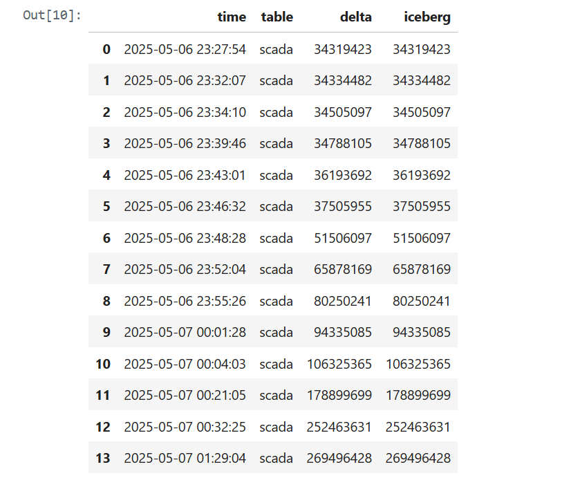
- Recording the record counts in a results table to track and visualize the comparison over time.
The results were quite awesome. I plotted the total record counts from both the Iceberg and Delta perspectives using two distinct colors and observed a perfect match. This confirms the seamless interoperability provided by XTable.
Lesson learned:
See the code snippet below for inserting data in Snowflake:
snow.execute(f'insert into ONELAKE.ICEBERG.scada select * from ONELAKE.AEMO.SCADARAW limit {limit};')
snow.execute('delete from ONELAKE.ICEBERG.scada where INITIALMW = 0')
snow.execute("SELECT SYSTEM$GET_ICEBERG_TABLE_INFORMATION('ONELAKE.iceberg.scada');")
In rare cases—especially when running multiple transactions at the same time—Snowflake may not instantly generate the metadata. To be 100% sure, run this SQL statement
SELECT SYSTEM$GET_ICEBERG_TABLE_INFORMATION('Table_name')to force the engine to write new Iceberg metadata. It’s an annoying aspect of Iceberg: every commit generates three files. That’s a bit excessive. Some engines prefer to group multiple commits to reduce the size of the metadata. Again, it’s rare—but it does happen.
]]>TL;DR
I built a simple Fabric Python notebook to orchestrate sequential SQL transformation tasks in OneLake using DuckDB and delta-rs. It handles task order, stops on failure, fetches SQL from external sources (like GitHub or a Onelake folder), manages Delta Lake writes, and uses Arrow recordbacth for efficient data transfer, even for large datasets. This approach helps separate SQL logic from Python code and simulates external table behavior in DuckDB. Check out the code on GitHub: https://github.com/djouallah/duckrun
pip install duckrunIntroduction
Inspired by tools like dbt and sqlmesh, I started thinking about building a simple SQL orchestrator directly within a Python notebook. I was showing a colleague a Fabric notebook doing a non-trivial transformation, and although it worked perfectly, I noticed that the SQL logic and Python code were mixed together – clear to me, but spaghetti code to anyone else. With Fabric’s release of the user data function, I saw the perfect opportunity to restructure my workflow:
- Data ingestion using a User-Defined Function (UDF), which runs in a separate workspace.
- Data transformation in another workspace, reading data from the ingestion workspace as read-only.
- All transformations are done in pure SQL, there 8 tables, every table has a sql file, I used DuckDB, but feel free to use anything else that understands SQL and output arrow (datafusion, chdb, etc).
- Built Python code to orchestrate the transformation steps.
- PowerBI reports are in another workspace
I think this is much easier to present

I did try yato, which is a very interesting orchestrator, but it does not support parquet materialization
How It Works
The logic is pretty simple, inspired by the need for reliable steps:
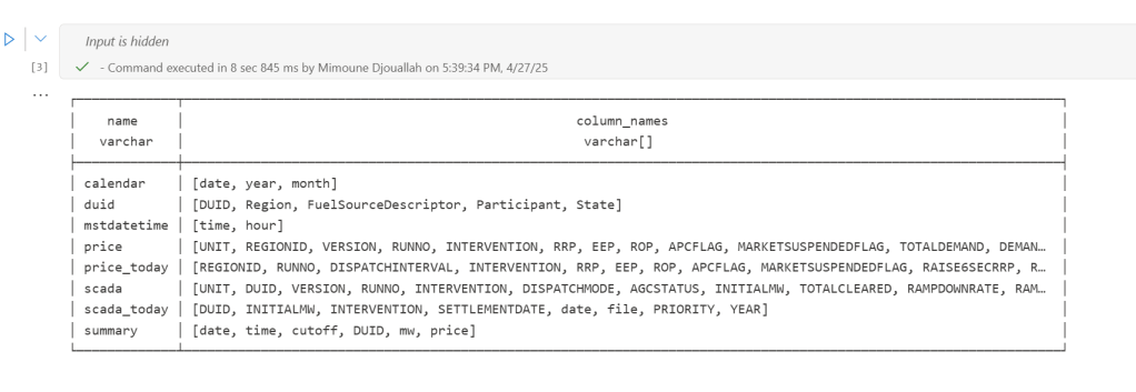
- Your Task List: You provide the function with a list (tasks_list). Each item has table_name (same SQL filename, table_name.sql) and how to materilize the data in OneLake (‘append’ , ‘overwrite’,ignore and None)
- Going Down the List: The function loops through your tasks_list, taking one task at a time.
- Checking Progress: It keeps track of whether the last task worked out using a flag (like previous_task_successful). This flag starts optimistically as True.
- Do or Don’t: Before tackling the current task, it checks that flag.
- If the flag is True, it retrieves the table_name and mode from the current task entry and passes them to another function, likely called run_sql. This function performs the actual work of running your transformation SQL and writing to OneLake.
- If the flag is False, it knows something went wrong earlier, prints a quick “skipping” message, and importantly, uses a break statement to exit the loop immediately. No more tasks are run after a failure.
- Updating the Status: After run_sql finishes, run_sql_sequence checks if run_sql returned 1 (our signal for success). If it returns 1, the previous_task_successful flag stays True. If not, the flag flips to False.
- Wrap Up: When the loop is done (either having completed all tasks or broken early), it prints a final message letting you know if everything went smoothly or if there was a hiccup.
The run_sql function is the workhorse called by run_sql_sequence. It’s responsible for fetching your actual transformation SQL (that SELECT … FROM raw_table). A neat part here is that your SQL files don’t have to live right next to your notebook; they can be stored anywhere accessible, like a GitHub repository, and the run_sql function can fetch them. It then sends the SQL to your DuckDB connection and handles the writing part to your target OneLake table using write_deltalake for those specific modes. It also includes basic error checks built in for file reading, network stuff, and database errors, returning 1 if it succeeds and something else if it doesn’t.
You’ll notice the line con.sql(f””” CREATE or replace SECRET onelake … “””) inside run_sql; this is intentionally placed there to ensure a fresh access token for OneLake is obtained with every call, as these tokens typically have a limited validity period (around 1 hour), keeping your connection authorized throughout the sequence.
When using the overwrite mode, you might notice a line that drops DuckDB view (con.sql(f’drop VIEW if exists {table_name}’)). This is done because while DuckDB can query the latest state of the Delta Lake files, the view definition in the current session needs to be refreshed after the underlying data is completely replaced by write_deltalake in overwrite mode. Dropping and recreating the view ensures that subsequent queries against this view name correctly point to the newly overwritten data.
The reason we do this kind of hacks is, duckdb does not support external table yet, so we are just simulating the same behavior by combining duckdb and delta rs, spark obviousely has native support
Handling Materialization in Python
One design choice here is handling the materialization strategy (whether to overwrite or append data) within the Python code (run_sql function) rather than embedding that logic directly into the SQL scripts.
Why do it this way?
Consider a table like summary. You might have a nightly job that completely recalculates and overwrites the summary table, but an intraday job that just appends the latest data. If the overwrite or append command was inside the SQL script itself, you’d need two separate SQL files for the exact same transformation logic – one with CREATE OR REPLACE TABLE … AS SELECT … and another with INSERT INTO … SELECT ….
By keeping the materialization mode in the Python run_sql function and passing it to write_deltalake, you can use the same core SQL transformation script for the summary table in both your nightly and intraday pipelines. The Python code dictates how the results of that SQL query are written to the Delta Lake table in OneLake. This keeps your SQL scripts cleaner, more focused on the transformation logic itself, and allows for greater flexibility in how you materialize the results depending on the context of your pipeline run.
Efficient Data Transfer with Arrow Record batch
A key efficiency point is how data moves from DuckDB to Delta Lake. When DuckDB executes the transformation SQL, it returns the results as an Apache Arrow RecordBatch. Arrow’s columnar format is highly efficient for analytical processing. Since both DuckDB and the deltalake library understand Arrow, data transfers with minimal overhead. This “zero-copy” capability is especially powerful for handling datasets larger than your notebook’s available RAM, allowing write_deltalake to process and write data efficiently without loading everything into memory at once.
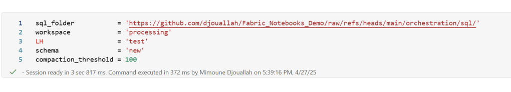
Example:
you pass Onelake location, schema and the number of files before doing any compaction
first it will load all the existing Delta table
Here’s an example showing how you might define and run different task lists for different scenarios:
sql_tasks_to_run_nightly = [
    ['price', 'append'],
    ['scada', 'append'],
    ['duid', 'ignore'],
    ['summary', 'overwrite'], # Overwrite summary nightly
    ['calendar', 'ignore'],
    ['mstdatetime', 'ignore'],
]

sql_tasks_to_intraday = [
    ['price_today', 'append'],
    ['scada_today', 'append'],
    ['duid', 'ignore'],
    ['summary', 'append'] # Append to summary intraday using the *same* SQL script
]
You can then use Python logic to decide which pipeline to run based on conditions, like the time of day:
start = time(4, 0)
end = time(5, 30)

if start <= now_brisbane <= end:
    run_sql_sequence(sql_tasks_to_run_nightly)
Here’s an example of an error I encountered during a run, it will automatically stop the remaining tasks:
Attempting to run SQL for table: price_today with mode: append
Running in mode: append for table: price_today
Error writing to delta table price_today in mode append: Parser Error: read_csv cannot take NULL list as parameter
Error updating data or creating view in append mode for price_today: Parser Error: read_csv cannot take NULL list as parameter
Failed to run SQL for table: price_today. Stopping sequence.
One or more SQL tasks failed.
here is some screenshots from actual runs
as it is a delta table, I can use SQL endpoints to get some stats
For example the table scada has nearly 300 Million rows, the raw data is around 1 billion of gz.csv

It took nearly 50 minutes to process using 2 cpu and 16 GB of RAM, notice although arrow is supposed to be zero copy, writing parquet directly from Duckdb is substantially faster !!! but anyway, the fact it works at all is a miracle
in the summary table we remove empty rows and other business logic, which reduce the total size to 119 Million rows.
here is an example report using PowerBI direct lake mode, basically reading delta directly from storage
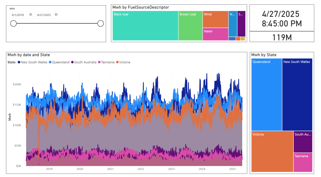
In this run, it did detect that the the night batch table has changed

Conclusion
To be clear, I am not suggesting that I did anything novel, it is a very naive orchestrator, but the point is I could not have done it before, somehow the combination of open table table format, robust query engines and an easy to use platform to run it make it possible and for that’s progress !!!
I am very bad at remembering python libraries syntax but with those coding assistants, I can just focus on the business logic and let the machine do the coding. I think that’s good news for business users.
]]>By now, it’s become clear that Parquet is the de facto standard for storing data, and using an object store to separate storage from compute makes a lot of sense.
Another interesting development is how vendors want to package this offering. Storage vendors saw an opportunity to do more—after all, there’s no law that says the metastore belongs to the data warehouse! So you get things like S3 Table and Cloudflare R2, which I think is a good thing, especially if you’re a smaller analytics vendor. Life becomes much easier when table maintenance is done upstream, allowing you to focus solely on making the query engine faster.
Encouraging things are also happening in the table format space. I know a bit about Iceberg and Delta, but not much about the others. One very interesting development is Iceberg adopting deletion vectors from Delta in the V3 spec, while Delta will requires a catalog for read and write (at least for catalog managed table). I like to call it the “Icebergification” of Delta.
Another trend is the Delta Java writer making it easier to auto-generate Iceberg metadata. and Xtable is doing the same regardless of the delta writer, At this stage, one could argue: why do we need two table formats that are becoming virtually identical?
Data Analyst—How About Me?
These improvements mostly impact the write path, which is primarily managed by data engineers. But what about data analysts and end users?
if you have Fabric OneLake, you can use Direct Lake in OneLake mode. Marco has a great article about it. It’s a fantastic improvement compared to the initial version of Direct Lake. However, it doesn’t solve the problem if your data is hosted in an S3 table or BigQuery Iceberg table. Yes, you can create a shortcut to OneLake and read it from there, but that still depends on a data engineer setting it up.
Now imagine a world where an Excel, Tableau, or Power BI Desktop user (or any arbitrary client tool) can just point to a Lakehouse using a standard API, discover tables, read data, and build reports. Honestly, this isn’t a big ask , we already have this when connecting to databases using ODBC, and I don’t see any technical reason why we can’t have the same experience with Lakehouses.
We Already Have This API
For me, the most promising development in the Lakehouse ecosystem is the Iceberg Catalog REST API, and I genuinely hope it becomes a standard—just like ODBC is today (and hopefully ADBC in the future, but that’s another topic).
Again, speaking as a data analyst, I want my tools to support the read part of the API—just the ability to list tables and scan a table. That’s all. I have zero interest in how the data is stored or which table format is used. The catalog should be smart enough to generate metadata on the fly.
The Good News
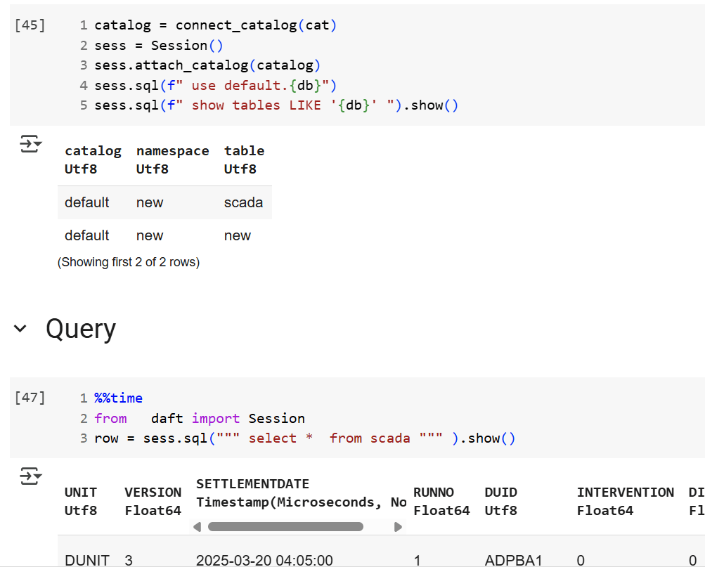
We’re getting there—at least if you’re using a Python notebook. Here’s an example where I use the same Iceberg REST API to query a table from four different Lakehouse implementations using Daft.
def connect_catalog(cat):
  match cat:
    case 'polaris':
      catalog = load_catalog(
              'default',
              uri= polaris_endpoint,
              warehouse='dwh',
              scope = 'PRINCIPAL_ROLE:data_engineer' ,
              credential= polaris_key
            )
    case 's3':
      catalog = load_catalog(
              'default',
              **{
                "type": "rest",
                "warehouse": s3_warehouse ,
                "uri": "https://s3tables.us-east-2.amazonaws.com/iceberg",
                "rest.sigv4-enabled": "true",
                "rest.signing-name": "s3tables",
                "rest.signing-region": "us-east-2"
              }
            )
    case 'uc':
      catalog = load_catalog(
               'default',
              token = token ,
              uri = endpoint,
              warehouse = 'ne'
              )
    case 'r2':
      catalog = RestCatalog(
              name = 'default',
              token = token_r2 ,
              uri = endpoint_r2,
              warehouse = r2_warehouse
              )
  return catalog
Then, I run a standard SQL query using Daft SQL.
Final Thoughts
It took Parquet a decade to become a standard. We may or may not have a single standard table format—and maybe we don’t need one. But if we want this Lakehouse vision to become mainstream, then everyone should support the Iceberg Catalog REST API, at least for read operations.
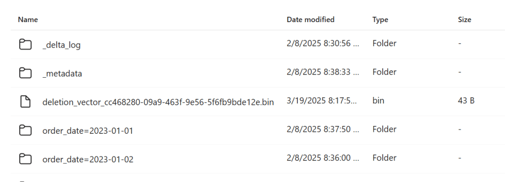
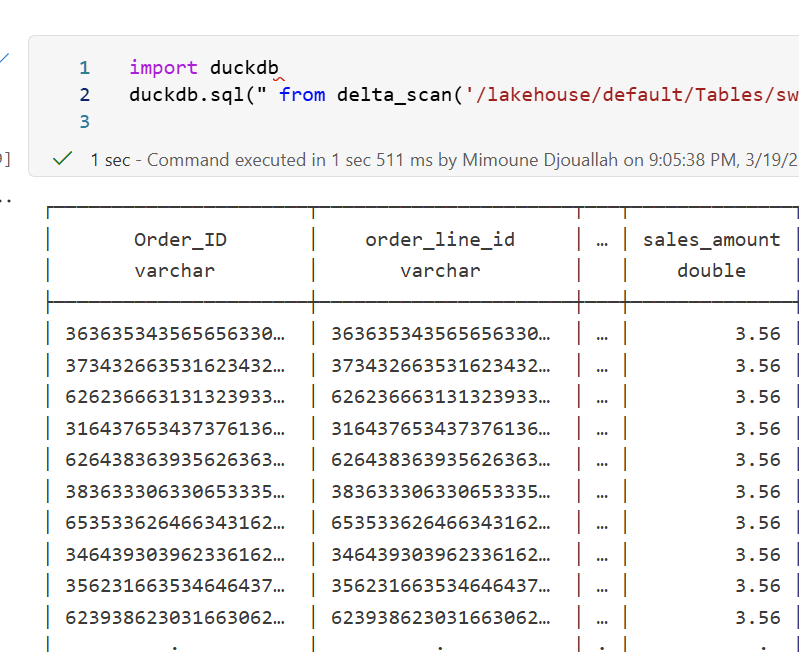
]]>deltalake library (Delta_rs, not Spark), you may encounter the following error:
import deltalake

DeltaTable('/lakehouse/default/Tables/xxx').to_pyarrow_dataset()
DeltaProtocolError: The table has set these reader features: {'deletionVectors'} but these are not yet supported by the deltalake reader.
Alternative: Using DuckDB
A simple alternative is to use DuckDB:
import duckdb

duckdb.sql("SELECT COUNT(*) FROM delta_scan('/lakehouse/default/Tables/xxx')")
Tested with a file that contains Deletion vectors
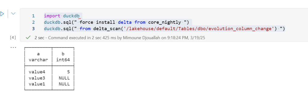
Column Mapping
The same approach applies to column mapping as well.
Upgrading DuckDB
Currently, Fabric Notebook comes preinstalled with DuckDB version 1.1.3. To use the latest features, you need to upgrade to the latest stable release (1.2.1) :
!pip install duckdb --upgrade
import sys
sys.exit(0)
Note: Installing packages using
%pip installdoes not restart the kernel when you run the notebook , you need to usesys.exit(0)to apply the changes, as some packages may already be loaded into memory.
import duckdb
duckdb.sql(" force install delta from core_nightly ")
duckdb.sql(" from delta_scan('/lakehouse/default/Tables/dbo/evolution_column_change') ")
The Future of Delta Rust .
Currently, there are two Rust-based implementations of Delta:
- Delta_rs: The first and more mature implementation, developed by the community. It is an independent implementation of the Delta protocol and utilizes DataFusion and PyArrow (which will soon be deprecated) as its engine. However, Delta_rs does not support deletion vectors or column mapping, though it does support writing Delta tables.
- Delta Kernel_rs: The newer, “official” implementation of Delta, providing a low-level API for query engines. It is currently being adopted by DuckDB ( and Clickhouse apparently) with more engines likely to follow. However, it is still a work in progress and does not yet support writing.
There are ongoing efforts to merge Delta_rs with Delta Kernel_rs to streamline development and reduce duplication of work.
Note : although they are written in Rust, we mainly care about the Python API
Conclusion
At least for now, in my personal opinion, the best approach is to:
- Use DuckDB for reading Delta tables
- Use Python Deltalake (Delta_rs) for writing
Before proceeding, ensure you have the necessary tools installed and configured. For more details, refer to the official installation guide: Install Azure CLI on Windows.
- Install Azure CLI (one-time setup)
winget install Microsoft.AzureCLIEnsure you have the latest version installed. - Login to Azure
az loginFollow the browser-based authentication flow.
Installing Required Python Package
The obstore package is a Python API for the Rust-based Object Store crate, which simplifies interaction with cloud storage systems.
pip install obstore --upgrade
Connecting to OneLake Storage
Once installed, you can connect to OneLake using the obstore package:
import obstore
from obstore.store import from_url

# Define storage path
store = from_url('abfss://[email protected]/power.Lakehouse/Files', azure_use_azure_cli=True)
there is a PR by someone from the community where azure_use_azure_cli=True will not be needed the system will automatically pick the available authentification
Listing Files in OneLake
To list the files and folders inside OneLake, always specify a prefix to avoid long processing times:
obstore.list(store, 'tmp').collect()

Uploading Local Files to OneLake
To upload files from a local directory to OneLake, use the following script:
import os

folder_path = '/test'  # Change this to the directory containing your files

for root, dirs, files in os.walk(folder_path):
    for file in files:
        local_path = os.path.join(root, file).replace("\\", "/")
        print(f"Uploading: {local_path}")
        obstore.put(store, local_path, local_path)


Downloading Files
for downloading files, you use get
xx = obstore.get(store,'plan/plan.png').bytes()
with open('output_file.png', 'wb') as file:
    file.write(xx)
Compatibility with Other Storage Solutions
The beauty of this approach is that the code remains largely the same whether you’re using OneLake or an S3-compatible storage service. The main differences lie in updating:
- The storage path
- Authentication credentials
Note: OpenDale provides a similar solution, but it does not currently support Entra OAuth 2
Summary
This short blog outlines a straightforward way to load files into OneLake using Python. With Azure CLI authentication and obstore, managing files in OneLake becomes both simple and specially standardized.
Obviously, it was always possible to do the same using Azure storage SDK but, the API is far from being user friendly (Personal opinion), it is designed for developers, but as a business user I like this package
Thanks Kyle Barron for creating this package
You can download a sample notebook here :
]]>If you’ve ever worked with Delta tables, for example using delta_rs, you know that writing to one is as simple as passing the URL and credentials. It doesn’t matter whether the URL points to OneLake, S3, Google Cloud, or any other major object store — the process works seamlessly. The same applies whether you’re writing data using Spark or even working with Iceberg tables.
However, things get complicated when you try to list a bucket or copy a file. That’s when the chaos sets in. There is no standard method for these tasks, and every vendor has its own library. For instance, if you have a piece of code that works with S3, and you want to replicate it in Azure, you’ll need to rewrite it from scratch.
This is where OpenDal comes in. OpenDal is an open-source library written in Rust (with Python bindings) that aims to simplify this problem. It provides a unified library to abstract all object store primitives, offering the same API for file management across multiple platforms (or “unstructured data” if you want to sound smart). While the library has broader capabilities, I’ll focus on this particular aspect for now.
I tested OpenDal with Azure ADLS Gen2, OneLake, and Cloudflare R2. To do so, I created a small Python notebook (with the help of ChatGPT) that syncs any local folder to remote storage. It works both ways: if you add a file to the remote storage, it gets replicated locally as well.
Currently, there’s a limitation: OpenDal doesn’t work with OneLake yet, as it doesn’t support OAuth tokens, and SAS tokens have a limited functionality ( it is by design, you can’t list a container for example from OneLake)
You can download the notebook here
Here’s an example of how it works:
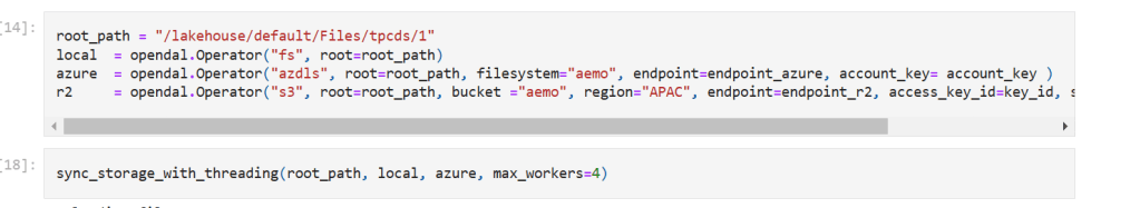
you need just to define your object store and the rest is the same, list, create folder, copy, write etc all the same !!! this is really a very good job
you can see the presentation but it is too technical to my taste https://www.youtube.com/watch?v=eVMIzY1K5iQ
Local folder :

Cloudflare R2:


Notice; I am using lakehouse mounted storage, for a background on the different access mode, you can read the previous blog
Data Generation Challenges
Initially, I encountered an out-of-memory error while generating the dataset. Upgrading to the development release of DuckDB resolved this issue. However, the development release currently lacks support for reading Delta tables, as Delta functionality is provided as an extension available only in the stable release.
Here are some workarounds:
- Increase the available RAM.
- Use the development release to generate the data, then switch back to version 1.1.3 for querying.
- Wait for the upcoming version 1.2, which should resolve this limitation.
The data is stored as Delta tables in OneLake, it was exported as a parquet files by duckdb and converted to delta table using delta_rs (the conversion was very quick as it is a metadata only operation)
Query Performance
Running all 99 TPC-DS queries worked without errors, albeit very slowly( again using only 2 cores ).
I also experimented with different configurations:
4, 8, and 16 cores: Predictably, performance improved as more cores were utilized.
For comparison, I ran the same test on my laptop, which has 8 cores and reads my from local SSD storage, The Data was generated using the same notebook.
Results
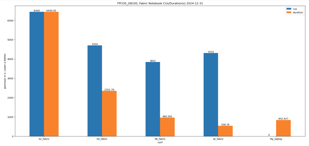
Python notebook compute consumption is straightforward, 2 cores = 1 CUs, the cheapest option is the one that consume less capacity units, assuming speed of execution is not a priority.
- Cheapest configuration: 8 cores offered a good balance between cost and performance.
- Fastest configuration: 16 cores delivered the best performance.
Interestingly, the performance of a Fabric notebook with 8 cores reading from OneLake was comparable to my laptop with 8 cores and an SSD. This suggests that OneLake’s throughput is competitive with local SSDs.
Honestly, It’s About the Experience
At the end of the day, it’s not just about the numbers. There’s a certain joy in using a Python notebook—it just feels right. DuckDB paired with Python creates an intuitive, seamless experience that makes analytical work enjoyable. It’s simply a very good product.
Conclusion
While this experiment may not have practical applications, it highlights DuckDB’s robustness and adaptability. Running TPC-DS with such limited resources showcases its potential for lightweight analytical workloads.
You can download the notebook for this experiment here:
]]>