Editors’ Highlights are summaries of recent papers by AGU’s journal editors.

Source: AGU Advances

Many are impressed by the power of artificial intelligence (AI) and its astonishing capability to make a synthesis of information. But, what we don’t realize is the price that we have to pay in terms of environmental impact for the development of AI.

Privette et al. [2026] assess the multi-faceted water footprint of data centers that make the necessary calculations to empower AI. Their commentary claims more transparency is necessary for communicating the water usage of data centers, and for supporting effective regulation and community planning. Ensuring the sustainability of data centers in the face of growing needs requires a cooperative effort by public administrations, industrial sector and communities of users. The authors emphasize that rigorous monitoring of environmental impact indicators is necessary to ensure that AI effectively supports the progress of our knowledge.

Citation: Privette, A. P., Barros, A., & Cai, X. (2026). Data centers water footprint: The need for more transparency. AGU Advances, 7, e2025AV002140. https://doi.org/10.1029/2025AV002140

—Alberto Montanari, Editor-in-Chief, AGU Advances

Text © 2026. The authors. CC BY-NC-ND 3.0
Except where otherwise noted, images are subject to copyright. Any reuse without express permission from the copyright owner is prohibited.

Far below the ocean’s sunlit surface, there are places in the water where oxygen runs low, sometimes becoming so depleted that barely any remains. These regions, called oxygen minimum zones (OMZs), are vast midwater deserts that make survival difficult for many organisms: Fish migrate elsewhere, and shell-forming microscopic species begin to dissolve. Yet deserts are never lifeless, and within OMZs, microbial life thrives.

Throughout most of the ocean, aerobic bacteria use dissolved molecular oxygen to decompose organic matter and gain energy, releasing carbon dioxide in the process. But when water ages or is overloaded with organic material, this oxygen is completely consumed, and OMZs become oxygen-deficient zones (ODZs).

In the absence of dissolved oxygen, anaerobic microbes take over, stripping oxygen atoms from other molecules like nitrate (a key nutrient for photosynthesis in the sunlit ocean) to consume organic matter and transforming those molecules step by step into nitrogen gas that can eventually escape to the atmosphere. As a result, ODZs are hot spots of nitrogen loss from the ocean, loss that subtly, but significantly, alters the marine nitrogen reservoir that sustains global productivity and the carbon cycle.

Strongest in the tropical Pacific and Indian Oceans (but also occurring in the Atlantic), OMZs are expanding—and their ODZ cores are intensifying—as warmer and more stratified waters slow oxygen replenishment from the surface (Figure 1).

To predict how OMZs and ODZs will evolve, scientists must observe the invisible chemistry that drives them—chemistry that has been nearly impossible to measure across seasons, years, and vast areas of the ocean. With a newly developed technique inspired by bioinformatics software, however, I have begun unmasking a crucial chemical signal long hidden in existing oceanic datasets. Applying this technique to data old and new will help researchers reveal important details of nitrogen cycling and other secrets of the ocean.

The Challenges of Measuring Transient Molecules

OMZs are notoriously difficult to study. Nitrogen transformations within these zones occur through multistep reactions driven by different cohorts of specialized microbes. The microbes generate fleeting, intermediate molecules that react quickly before reaching their final form as nitrogen gas. Among the most important of these is nitrite, which acts as a “control valve on the marine N [nitrogen] budget,” and nitrous oxide, a potent greenhouse gas that can escape to the atmosphere before being converted into nitrogen gas.

Understanding how marine microbes transform nitrate into various intermediates and eventually into nitrogen requires frequent measurements of molecular concentrations at sea to capture the rapid reactions. Observations must also be collected across different depths, as distinct microbial communities inhabit specific water layers, causing these processes to vary spatially. These requirements create substantial challenges to adequate ocean sampling.

Ship-based sampling is valuable but sparse across space and time, meaning it is often insufficient for detecting how transient molecules in nitrogen transformation processes are produced and consumed in situ.

Robotic platforms that drift, dive, and surface across the global ocean offer another option. In particular, the system of biogeochemical Argo (BGC-Argo) floats, which record and return data around the clock and in near-real time, comprises a worldwide network of hundreds of remote observers that continuously measure nitrate, oxygen, pH, and other ocean properties.

Until recently, these autonomous sensors were thought to be blind to short-lived nitrite, the key to revealing how microbes in oxygen-deficient waters regulate the planet’s nitrogen and carbon cycles. Now, however, oceanographers can rely on them for measurements of this all-important intermediary [Bif and Johnson, 2025].

A Statistical Spark

When I began working at the Monterey Bay Aquarium Research Institute (MBARI), a casual conversation with my former supervisor Ken Johnson about ocean floats changed the course of my research. He mentioned that the data from nitrate sensors on floats might already contain hidden information about nitrite. These sensors measure oceanic nitrate indirectly by detecting how strongly ultraviolet (UV) light at specific wavelengths is absorbed by seawater.

Like nitrate, nitrite also absorbs UV light because of its inherent chemical characteristics, albeit more weakly. And from float data collected in ODZs, where nitrite is known to be present, it appeared that nitrite might, indeed, be altering detected UV spectral signals from what’s expected from nitrate alone. However, when Ken had tried to add nitrite as an extra variable into his calculations of nitrite and nitrate concentrations, the results did not match observed real-world measurements; the calculated values were simply too high for the ocean. Curiosity over that discrepancy became our starting point for further digging.

I began investigating the spectral fingerprints of compounds commonly found in ODZs, including nitrite. In the lab, I mixed these compounds into seawater and used the same UV spectrometers deployed on BGC-Argo floats to test their UV absorption. Among the molecules studied, nitrite and thiosulfate (an intermediate compound in the much less known sulfur cycle) were the strongest absorbers. Each left a subtle but distinct imprint on the UV spectrum. If those spectral signatures—hidden within what had long been considered noise—could be teased apart statistically, it might be possible to detect these fleeting intermediates in the ocean remotely.

The evidence was there, but we had to find a way to separate the signals from those of compounds that often coexist inside ODZs. That breakthrough happened with assistance from an unexpected source: Ken’s brother, Bruce Johnson, a bioinformatics researcher at the City University of New York’s Advanced Science Research Center.

Over dinner with Ken while he was in town for a conference near MBARI, Bruce described an upgrade to the software he develops to determine protein structures from nuclear magnetic resonance spectral data. The upgrade involves using a statistical approach called LASSO (Least Absolute Shrinkage and Selection Operator) regression to sift through overlapping chemical signals and identify the key components behind a spectrum. If it works for parsing different protein structures, Ken thought, maybe we could use it to sort molecular signals in our UV spectra. I loved the idea.

And it worked. After building our own algorithms to apply LASSO regression, we could finally separate the faint spectral contributions of nitrite and thiosulfate from the much stronger nitrate signal. What began as a speculative idea born from a cross-disciplinary family conversation became a powerful analytical tool. The next question was whether the ocean would confirm what our mathematical calculations and experimental lab data had revealed.

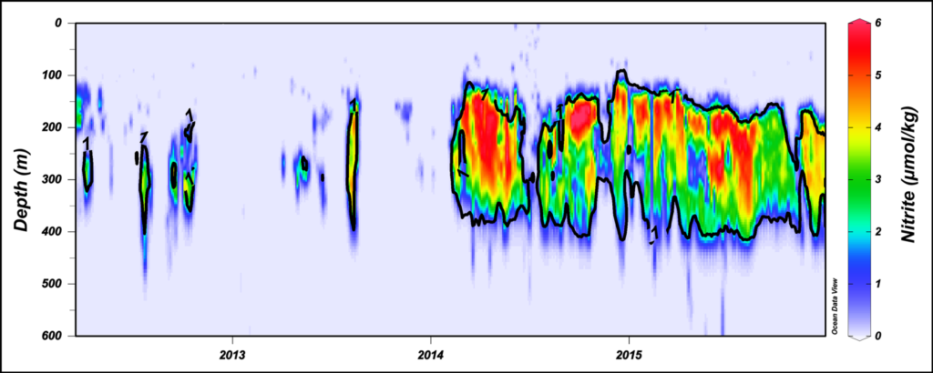
Indeed, it did. Applying the LASSO method to real BGC-Argo float data collected at different ODZs, we watched nitrite patterns emerge for the first time from years of raw spectra, even those from older floats that have long since stopped operating [Bif and Johnson, 2025] (Figure 2). Analysis of research cruise water samples validated the signals seen in the float data, confirming that they’d been recording chemical transformations all along. Seeing the first time series of nitrite concentration data gave the impression that the ocean was speaking back to us, revealing a story long hidden from view.

What the Ocean May Tell Us

The ability to measure nitrite in seawater allows us to track nitrogen (and potentially sulfur) transformations remotely and continuously and to connect biochemical microbial processes to large-scale cycling of elements in the ocean. With this approach, for example, we can now examine vast datasets to map how nitrogen cycling changes across seasons and years and to identify the chemical processes occurring within different layers of an ODZ.

Perhaps most exciting is that so many datasets already exist. By reanalyzing UV spectra from sensors deployed on BGC-Argo floats, we are uncovering new information about ocean chemistry. Building on this effort, we are applying a biochemical model to estimate reaction rates of microbially mediated nitrogen transformations [Bif et al., 2025], bridging the gap between chemical observations and the biological processes that control them.

To further strengthen and validate the approach, we are collecting new data to survey additional ODZs, including during recent field campaigns in the Bay of Bengal in June–August 2025 and the Santa Barbara Basin in October 2025. In parallel, we are developing a new method to automate measurement of sulfite and thiosulfate concentrations in situ, providing a crucial link between laboratory measurements and float-based observations of the sulfur cycle.

Floating Into the Future

The advances highlighted here came from curiosity and persistence and reveal the power of interdisciplinary thinking—in this case involving chemistry, biology, and engineering applied to oceanography. They also show the potential to further tap existing arrays of scientific ocean floats to reveal even more about the invisible ocean than they already do.

We didn’t invent new sensors for the floats; we just learned to use the tools at our disposal differently. As this capability is applied globally, it will enable the oceanographic community to better constrain nitrogen transformation processes that have long been difficult to observe directly.

Of course, to keep learning, we need instruments in the water. The future availability of the global BGC-Argo network, which made these discoveries possible, and other floats is in question given the uncertainty of long-term support for float maintenance and new deployments both in the United States and internationally. Our ability to observe the ocean’s invisible chemistry and the microbial transformations that drive elemental cycles could thus fade just as vital signals are coming into focus.

The ocean still holds many secrets in OMZs and elsewhere that affect us globally and locally. Maintaining the tools we have—and finding innovative ways to use them—is an efficient strategy for leveraging investments already made as we look to reveal these secrets.

References

Bif, M. B., and K. S. Johnson (2025), BGC-Argo floats reveal nitrite and thiosulfate dynamics in the oceans with high spatiotemporal resolution, Global Biogeochem. Cycles, 39, e2024GB008473, https://doi.org/10.1029/2024GB008473.

Bif, M., et al. (2025), BGC-Argo float reveals regime shifts in nitrogen-carbon cycling in an oxygen-deficient zone, Research Square, https://doi.org/10.21203/rs.3.rs-7809237/v1.

Author Information

Mariana Bif ([email protected]), Rosenstiel School of Marine, Atmospheric and Earth Sciences, University of Miami, Key Biscayne, Fla.

Citation: Bif, M. (2026), A new twist on robotic float data reveals critical ocean chemistry, Eos, 107, https://doi.org/10.1029/2026EO260086. Published on 18 March 2026.

Text © 2026. The authors. CC BY-NC-ND 3.0
Except where otherwise noted, images are subject to copyright. Any reuse without express permission from the copyright owner is prohibited.

Editors’ Vox is a blog from AGU’s Publications Department.

Frozen soil covers about 20% of the Earth’s land surface, and acts like a seasonal or long-term underground dam that controls how water moves and how carbon is stored. A new article in Reviews of Geophysics explores recent advances in the physics, observation, and modeling of frozen soil hydrology. Here, we asked the lead author to give an overview of frozen soil, how climate change is expected to influence it, and directions for future research.

Approximately how much of the Earth’s surface is comprised of frozen soil and where does it occur?

Frozen soil includes both permafrost, which remains frozen for at least two consecutive years, and seasonally frozen ground, which freezes and thaws each year. Together, these frozen landscapes affect roughly one-fifth of Earth’s land surface and much of the Northern Hemisphere. Permafrost is common in Arctic and sub-Arctic regions such as Alaska, northern Canada, Siberia, and Greenland, and it also occurs in high mountain and plateau regions, including the Qinghai-Tibet Plateau. Seasonally frozen ground extends much farther south into temperate regions. Although frozen ground is often associated with remote tundra, it also occurs in places where people live, work, farm, and build infrastructure, making it important far beyond the Arctic.

Why is it important to understand the hydrology of frozen soil?

Frozen ground strongly controls how water moves, where it is stored, and when it is released. In many cold regions, it behaves like a seasonal or long-term underground dam. When soils are frozen, ice can block pores, limit infiltration, and force meltwater to move laterally across the surface, which can increase spring runoff, erosion, and flooding. When thaw deepens, new pathways can open, allowing more recharge, stronger groundwater connectivity, and higher cold-season baseflow. These changes affect rivers, lakes, wetlands, water quality, ecosystems, and infrastructure. Understanding frozen-soil hydrology is therefore essential for predicting water resources and environmental change in cold regions under continued warming.

Why is it necessary to study frozen soil with an interdisciplinary approach?

Frozen-soil hydrology cannot be understood through hydrology alone. Whether water infiltrates, runs off, or moves through the subsurface depends on interactions among soil physics, heat transfer, vegetation, snow, groundwater, geochemistry, ecology, and engineering. Thaw can alter not only streamflow and groundwater recharge, but also carbon release, nutrient transport, wetland development, and infrastructure stability. Observations therefore need to combine field measurements, geophysics, remote sensing, and modeling across scales. An interdisciplinary approach helps link pore-scale freeze-thaw processes to landscape and watershed responses, while also connecting hydrologic change to broader impacts on ecosystems, climate feedbacks, and society.

How is climate change expected to influence frozen soil in the coming years?

Climate warming is already reducing the extent and duration of frozen ground in many regions. In permafrost areas, the active layer is becoming thicker and, in some places, year-round unfrozen zones known as taliks are forming beneath lakes, rivers, and thawed soils. In seasonally frozen regions, freezing periods are becoming shorter and less stable. These changes can either wet or dry landscapes, depending on topography, ground-ice content, and subsurface connectivity. In some Arctic lowlands, thaw promotes ponding, wetland expansion, and stronger winter flow. In other regions, especially some upland and plateau settings, deeper thaw can increase drainage and reduce near-surface soil moisture. The hydrologic response is therefore widespread but highly variable.

What are some recent advances that have improved our understanding of frozen soil hydrology?

Recent advances have greatly improved our understanding of frozen-soil hydrology. In the field, better sensors now measure soil temperature, moisture, thaw depth, and gas fluxes at higher resolution, while fiber-optic systems, drones, and geophysical methods help extend those observations across larger areas. Satellite products now capture freeze-thaw transitions, surface water changes, and land deformation associated with thaw. At the same time, models have improved their representation of phase change, unfrozen water, preferential flow, groundwater-permafrost interactions, and abrupt thaw. These advances are allowing researchers to connect small-scale freeze-thaw physics with broader watershed and regional responses, which is essential for predicting future cold-region hydrology under climate change.

What are some of the future directions for research identified in your review article?

Our review identifies several priorities for future research. First, we need stronger links between process studies, observations, and models so that pore-scale freeze-thaw physics can be represented more realistically at watershed and Earth-system scales. Second, more work is needed on threshold behavior, abrupt thaw, groundwater connectivity, and the changing seasonality of streamflow. Third, frozen-soil hydrology must be integrated more closely with carbon cycling, ecology, and infrastructure risk, because thaw affects all of these at the same time. Better long-term monitoring networks, shared datasets, and multi-method approaches that combine field measurements, geophysics, remote sensing, and modeling will be essential for reducing uncertainty and improving prediction.

—Ying Zhao ([email protected]; 0000-0003-0346-5631), Ludong University, China

Editor’s Note: It is the policy of AGU Publications to invite the authors of articles published in Reviews of Geophysics to write a summary for Eos Editors’ Vox.

Citation: Zhao, Y. (2026), How frozen ground controls water in a warming world, Eos, 107, https://doi.org/10.1029/2026EO265010. Published on 17 March 2026.

This article does not represent the opinion of AGU, Eos, or any of its affiliates. It is solely the opinion of the author(s).

Text © 2026. The authors. CC BY-NC-ND 3.0
Except where otherwise noted, images are subject to copyright. Any reuse without express permission from the copyright owner is prohibited.

For the first time in South America and only the sixth time in history, researchers have identified a field of tektites. Tektites, nicknamed space glass, are created when the intense heat generated by a cosmic collision with a meteorite melts silica-rich rocks on Earth’s surface. As the molten droplets cool down and fall back to the ground, they solidify into small pieces of glass.

Finding tektites is uncommon, but uncovering entire fields of these objects is even rarer. Up until now, such spots had been detected in only Australasia, central Europe, the Ivory Coast, North America, and, more recently, Belize. Some isolated glasses have also been found in the Atacama Desert in Chile and in Uruguay, but they were not recognized as fields.

“It is an interesting finding that adds probably the second additional tektite strewn field—besides the Belize one—to the four ‘classical’ fields that have been known for more than 100 years,” said Universität Wien impact researcher and geologist Christian Köberl, who did not take part in the study.

The discovery, described in the journal Geology, happened by chance when a resident of the Brazilian state of Minas Gerais reached out to scientists interested in meteorites to identify an unusual glass-like object he had found on his property. The object was sent to geologist Álvaro Penteado Crósta of Universidade Estadual de Campinas in São Paulo, who was initially skeptical that it could be a tektite.

“Tektites are extremely rare,” Crósta said. “They form under very specific conditions and do not survive long in the geological record. So it was a total surprise.”

Mounting Evidence

After he determined the piece was a tektite, Crósta received other specimens found dozens of kilometers away. That is when he decided to launch field trips to investigate further. In this effort, with the help of local residents, scientists collected around 500 glass pieces ranging in size from 1 to 6 centimeters and varying in shape from spherical to droplet shaped to twisted.

Although they appear black and opaque at first sight, the objects become translucent and display a grayish-green color under intense light.

Initially, the researchers identified a strewn field of tektites spanning a strip about 90 kilometers long in Minas Gerais, which is reported in the new paper. But after the study was submitted, new finds were identified in the states of Bahia and Piauí, extending the field across more than 900 kilometers.

According to Crósta, this puts the Brazilian tektite field in the midsize range: much smaller than the field in Australasia, which covers more than 10% of Earth’s surface, but similar in size to the field in western Belize.

But he thinks the Brazilian field could be even larger. “Now that the news is being spread, we might get contacted by more people with new samples,” said Crósta, adding that the new findings suggest that tektites may not be as rare as previously thought.

Isotopic analysis of the samples dated the Brazilian tektites, informally known as “geraisites” after the region where they were discovered, to 6.3 million years ago—relatively recent in geological terms.

Glassed from the Past

The new tektite findings can provide clues for scientists seeking to reconstruct the history of asteroid impacts on Earth. “The Earth was bombarded just like Mars,” Crósta said. “But here we do not see the craters as easily because our planet is very dynamic, with plate tectonics and erosion. To study this history, we must search for traces, and tektites are one of them.”

No crater associated with the impact that formed the Brazilian tektites has yet been found. Crósta thinks the crater could be buried and has begun searching for it using satellite imagery, geophysical data, and mathematical models. These tools, combined with paleomagnetic, geochemical, and isotope data, could help predict the location of the impact point. Currently, only nine meteorite craters have been recorded in Brazil, despite the country’s vast geography.

Köberl noted that it will be important to identify a possible source crater and determine how far the strewn field really extends to better understand the formation of tektites in general. “Six occurrences of different tektites worldwide are a rather small number,” he said. “This discovery adds important new observations and data to our understanding of tektites, but more analyses will be necessary.”

—Sofia Moutinho (@sofiamoutinho.bsky.social), Science Writer

17 March 2026: This article has been updated to correct an image credit.

Citation: Moutinho, S. (2026), Scientists discover South America’s first space glass fields, in Brazil, Eos, 107, https://doi.org/10.1029/2026EO260088. Published on 17 March 2026.

Text © 2026. The authors. CC BY-NC-ND 3.0
Except where otherwise noted, images are subject to copyright. Any reuse without express permission from the copyright owner is prohibited.

Children who live near gold mine tailings facilities in Johannesburg, South Africa, have nearly twice as much as uranium in their hair as those who don’t live near tailings facilities, according to new research. Concentrations were especially high in young children not yet attending school.

Uranium is present in most of the world’s soils in small amounts, so everyone is exposed to low levels of the metal. But exposure to higher levels of uranium and its decay products, such as radon, has been linked to kidney damage, neurological effects, and reduced lung function.

Unlike other heavy metals, such as zinc or iron, uranium “has no known benefit or metabolic function in the human body,” said Frank Winde, a geographer and environmental chemist at Wismut, a state-owned enterprise in Germany that is working to remediate uranium legacy sites. “[It] is only known to have adverse impacts on human health.”

Winde is a coauthor of a new paper on the findings, published in Environmental Geochemistry and Health.

Building Community Trust

The researchers worked with residents of three study sites within 3 kilometers of tailings facilities in Johannesburg: Riverlea, Tshepisong, and Snake Park, neighborhoods with a combined population of about 128,000 people. For reference sites, they worked with residents of Newlands East and Newlands West, two communities with a combined population of about 100,000 people located north of the city of Durban.

The team partnered with graduates from the University of Johannesburg and Mangosuthu University of Technology (located near Durban), as well as with local residents, to conduct fieldwork and hold a series of meetings with community members. They spent at least a month working to foster trust with the community, and hired at least one local resident for each fieldwork team.

Community representatives “had concerns about exposure to toxic substances from these mine tailings facilities, and some also expressed concerns about their health, and also their livestock,” said Busisiwe Shezi, a specialist scientist at the South African Medical Research Council (SAMRC) who studies exposure to environmental pollutants.

Some residents allowed the fieldwork team to sample soil from their yards, collect children’s hair samples of least 1 centimeter in length, and measure children’s height and weight. The residents also filled out questionnaires about the age, sex, and race of their children, as well as about how long they had lived in the area, whether they grew their own food at home, and other demographic data.

Researchers collected hair samples because hair can provide a record of an individual’s uranium exposure over 2–4 weeks, a period longer than that offered by blood or urine samples.

Michael Watts, a geochemist at the British Geological Survey, is the editor in chief of the journal in which the paper was published, but it was his co–editor in chief who reviewed the paper before publication. Watts told Eos that the researchers collected an appropriate amount of hair from each participant where possible (about 100 milligrams), which likely allowed the samples to be properly processed. He also noted that the researchers engaged with the community well and received appropriate commissions from the SAMRC Human Research Ethics Committee.

“It looks like a fantastic study,” Watts said. “It’s obviously gone through a lot of rigor in terms of planning and getting the permit.”

“Biomonitoring of vulnerable populations, particularly children, in regions impacted by legacy mining activities is a valuable and timely research focus,” said Matthew Omoniyi Isinkaye, an environmental scientist at Ekiti State University in Nigeria. However, he continued, “hair analysis for uranium exposure, while useful as a screening or indicative tool, is inherently subject to substantial uncertainties due to external contamination from dust and soil particles, which is very common, particularly in mine tailing environments.”

Smaller Bodies, Bigger Risks

The researchers sent 406 samples of hair (sealed in small, individual plastic bags) to Germany for testing. There, a team of scientists milled the hair, or ground it into a homogenized substance, explained Susanne Sachs, a chemist at the Institute of Resource Ecology–Helmholtz Zentrum Dresden Rossendorf who studies the environmental behavior of radionuclides.

“After that, this homogenized and milled hair was washed in order to remove any dust,” Sachs said. “This is in order to avoid any contaminations and to avoid overestimations of uranium concentrations.”

The team found that uranium concentrations were about twice as high in girls as in boys. This finding contrasts with previous studies that had found the opposite, signaling a need for more research into how biological sex influences the uptake and storage of toxins, the researchers said.

Hair from the 208 children from Johannesburg (the exposed group) had a median uranium concentration of 17.07 micrograms per kilogram, while hair from the 198 unexposed children from Durban had a concentration of 8.12 micrograms per kilogram. And the younger the children were, the higher the uranium concentrations in their hair: The geometric mean of uranium concentration was 0.99 times lower for each additional month of age.

The researchers weren’t surprised by this: Young children tend to touch their mouths more often, and some even eat soil. Not to mention, they’re simply smaller than their older counterparts.

“If you assume just identical volumes of uranium ingested with adults and kids, then having a much smaller body is already resulting in higher concentrations,” Winde said. However, he added, researchers don’t believe children are seeing the same exposure levels that adults are. “Actually, they have a higher uptake simply because they’re closer to where the stuff comes from. They play on the dumps. Some of them swim in the toe dams of tailings.”

Demographic data, including length of residence or water source, did not correlate significantly with detected levels of uranium.

Researchers did detect a difference in uranium concentrations in soil samples collected from exposed sites versus unexposed sites, but the difference was not as stark as the difference between hair samples. Shezi explained that a hair sample captures uranium taken up through multiple pathways, including by the inhalation of dust particles and the consumption of contaminated food or water.

“Whereas with soil, you’re just collecting a soil sample in one place at that one moment,” Shezi said.

Moving forward, the team hopes to return to the area, share their findings with the study participants, and conduct a longitudinal study of the risks of uranium exposure over time. Such research, the authors suggest, might contribute to stronger environmental protection and mitigation efforts around South Africa’s mining sites.

—Emily Gardner (@emfurd.bsky.social), Associate Editor

Citation: Gardner, E. (2026), Gold mines expose South African children to uranium, Eos, 107, https://doi.org/10.1029/2026EO260061. Published on 17 March 2026.

Text © 2026. AGU. CC BY-NC-ND 3.0
Except where otherwise noted, images are subject to copyright. Any reuse without express permission from the copyright owner is prohibited.

Editors’ Highlights are summaries of recent papers by AGU’s journal editors.

Source: Journal of Advances in Modeling Earth Systems

Today’s Earth System Models (ESMs) fail to inherently obey conservation laws such as total energy and therefore resort to ad hoc fixers to restore global balance. Without the latter, a spurious source of energy would contaminate signals like Earth’s energy imbalance in model simulations. Today’s ESMs also make simplifying and differing thermodynamic assumptions throughout the many components that collectively form an ESM. Designing and implementing an energetically and thermodynamically consistent ESM remains a grand challenge in weather and climate modeling.

The Climate Modeling Alliance (CliMA) has taken a considerable step in this direction by developing a novel fluid flow solver (a.k.a. dynamical core) with several new innovations addressing these decade-long consistency and conservation issues. Yatunin et al. [2026] use moist total energy as a prognostic variable with careful energetically consistent treatment of closure schemes and rigorous thermodynamics with minimal approximations and a modern efficient high-order numerical solver. The implementation in the Julia high-performance computing language ensures efficient execution on both CPU and GPU platforms.

Citation: Yatunin, D., Byrne, S., Kawczynski, C., Kandala, S., Bozzola, G., Sridhar, A., et al. (2026). The climate modeling alliance atmosphere dynamical core: Concepts, numerics, and scaling. Journal of Advances in Modeling Earth Systems, 18, e2025MS005014. https://doi.org/10.1029/2025MS005014

—Peter Lauritzen, Associate Editor, JAMES

This research is included in AGU’s Special Collection “The CliMA Earth System Model.”

Text © 2026. The authors. CC BY-NC-ND 3.0
Except where otherwise noted, images are subject to copyright. Any reuse without express permission from the copyright owner is prohibited.

Since 1968, there have been over 1,400 fatal landslides in Nepal, killing over 6,000 people.

I’m currently writing a paper on the patterns of fatal landslides in Nepal since 1968. This is an update on the paper we wrote almost 20 years ago (Petley et al. 2007) that examined the changing patterns of landslides there. This new paper reaches back rather further but also brings the analysis up to date.

As a part of this work, I have put together a dataset of fatal landslides. This is a hybrid – it incorporates a mixture of a long term study based on newspaper reports that was compiled in the DfID funded Landslide Risk Assessment in the Rural Access Sector project, my own data on global fatal landslides (which I’ve been compiling since 2003) and, more recently, the Nepali government dataset that is on the Bipad portal. Note that this dataset does not include seismically-triggered landslides.

As a result of this work, I have a chronology of fatal landslides – this is the pattern over this period:-

The main caveat here is the substantial change in methodology in about 2000, when data started to be collected in real time. This means that the data before that date probably underestimates the true impact. Thereafter, the data is likely to be quite consistent, but we do need to be alive to the impact of changing methodologies. Interestingly, though, there is some evidence that the dynamics of the monsoon changed in about 1996, when a marked increase in landslides is recorded.

Note the rising trend since 2000. It appears, although this needs further work, that there is a substantial increase in the number of fatal landslides in the most extreme years (this is when the monsoon is most intense). The three years with the largest number of fatal landslides have all occurred since 2020. There is also an apparent cyclicity in the data, but this may simply be an artefact or a coincidence.

The dataset includes 1,437 individual landslides that have claimed 6,195 lives. The data clearly shows both the rising impact of landslides in Nepal and the massive level of losses that they are imposing.

Reference

Petley, D.N., Hearn, G.J., Hart, A. et al. 2007. Trends in landslide occurrence in Nepal. Natural Hazards 43(1):23–44. https://doi.org/10.1007/s11069-006-9100-3

Text © 2026. The authors. CC BY-NC-ND 3.0
Except where otherwise noted, images are subject to copyright. Any reuse without express permission from the copyright owner is prohibited.

Research & Developments is a blog for brief updates that provide context for the flurry of news regarding law and policy changes that impact science and scientists today.

The University Corporation for Atmospheric Research (UCAR) filed a lawsuit today against the National Science Foundation (NSF), NOAA, the Department of Commerce (DOC), the Office of Management and Budget (OMB), and those agencies’ directors.

In December, the Trump administration announced plans to dismantle NSF’s National Center for Atmospheric Research (NCAR), which UCAR manages. NCAR, one of the world’s leading climate and Earth science research laboratories, is headquartered in Boulder, Colo.

The lawsuit alleges that the federal agencies are “waging a campaign of retaliation” against Colorado and its institutions because the state has not bowed to federal authorities. Namely, the state of Colorado prosecuted and convicted Tina Peters, the former County Clerk of Mesa County, for her efforts to overturn the results of the 2020 election, and Gov. Jared Polis refused President Trump’s order to grant Peters clemency. (The governor has since indicated he may reconsider.) The state has also not ended mail-in voting, a practice frequently criticized by the president.

“The Agencies have not identified any performance deficiency warranting adverse action, UCAR has remained in full compliance with the terms and conditions of its receipt of federal funding, and no agency has articulated a reasoned explanation for the coordinated effort to cripple UCAR and dismantle NCAR,” the lawsuit alleges. “That is because no such explanation exists.”

—Emily Gardner (@emfurd.bsky.social), Associate Editor

These updates are made possible through information from the scientific community. Do you have a story about how changes in law or policy are affecting scientists or research? Send us a tip at [email protected].

Text © 2026. AGU. CC BY-NC-ND 3.0
Except where otherwise noted, images are subject to copyright. Any reuse without express permission from the copyright owner is prohibited.

Editors’ Vox is a blog from AGU’s Publications Department.

Salt is a naturally occurring chemical compound that forms various types of evaporite minerals. These minerals precipitate in aqueous environments, such as shallow seas and lakes, and are of great significance to science and society.

A pair of two books recently published in AGU’s Geophysical Monograph Series covers recent advances in the study of salt. Salt in the Earth Sciences: Evaporite Rocks and Salt Deposition explores salt deposition and deformation in sedimentary basins, synthesizing data analysis, observations, theories, and modeling. Salt in the Earth Sciences: Basin Analysis and Salt Tectonics presents a global overview of giant salt basins formed across diverse tectonic settings, linking salt deposition to tectonic events, climate change, and more. We asked the author to tell us more about the books and why these topics matter.

Why is salt important to society?

Greek philosophers considered salt a vital element, together with earth, air, water, and fire. During the Medieval Ages, several nations traded salt as an important and extremely valuable commodity. And salt is just as significant today.

Salt production in the modern age has become an important industrial activity. For example, the chemical and fertilizer industries use several evaporite minerals to extract potassium. Lithium has been explored in salt basins in China and salt flats in Chile.

How do salt deposits relate to plate tectonics?

That’s an important question. Plate tectonic processes control salt deposition during two main phases: the first is the closure of oceanic basins due to plate convergence, which results in basins affected by compression; the other phase is the opening of oceanic basins during plate divergence, which creates rifts and continental margins separated by newly formed oceanic crust.

The first case is illustrated by the Persian Gulf region, which is characterized by salt basins that are currently under contraction due to the convergence of the Arabian and Asian plates. The South Atlantic illustrates the second case; rift basins with lacustrine environments developed in the early Cretaceous period, which in turn evolved into continental margins that are presently in the drift stage.

Climate is also an important factor controlling the formation of most salt basins. Salt deposition occurred under arid conditions when solar evaporation significantly exceeded precipitation, resulting in increased salinity in the gulfs that were open or closed by plate tectonics.

What are the two books about? Which geological periods and geographic regions do they cover?

The books concentrate on the significance of salt in the Earth sciences. They compare the fundamental principles of salt deposition, salt deformation, and the creation of halokinetic structures.

The books cover a wide range of sedimentary basins through geological time. The first recognized salt deposits on Earth are in the Precambrian region between Finland and Russia and in Central Africa. The book also discusses some examples of Neoproterozoic salt basins in Australia, which were involved in major orogenies during the Paleozoic. The region between the Arabian plate and the Eurasian plate hosts many important Neoproterozoic salt basins, particularly in the Persian Gulf and the Zagros region. The Neoproterozoic-to-Cambrian Hormuz salt is associated with major hydrocarbon discoveries in the Middle East.

Why should people read these books?        

The first volume not only offers a comprehensive review of the fundamental principles of deposition and deformation but also outlines the application of different geophysical methods used in the Earth sciences.

The second volume presents an overview of classical salt basins, including the Red Sea, the Central European region, the South Atlantic, the Mediterranean Sea, and the Gulf of Mexico. The second volume also presents an introduction to the future applications of the salt sciences in astrogeology and microbiology, discussing some extreme environments on Earth and other planets of the solar system.

Salt in the Earth Sciences: Evaporite Rocks and Salt Deposition, 2025. ISBN: 978-1-119-40521-4. List price: $225 (hardcover), $180 (e-book)

Salt in the Earth Sciences: Basin Analysis and Salt Tectonics, 2025. ISBN: 978-1-394-30703-6. List price: $225 (hardcover), $180 (e-book)

Chapter 1 of each book is freely available. Visit the books’ pages on Wiley.com and click on “Read an Excerpt” below the cover image.

—Webster Mohriak ([email protected]; 0000-0001-9254-685X), Rio de Janeiro State University, Brazil

Editor’s Note: It is the policy of AGU Publications to invite the authors or editors of newly published books to write a summary for Eos Editors’ Vox.

Citation: Mohriak, W. (2026), Salt: a vital compound for science and society, Eos, 107, https://doi.org/10.1029/2026EO265009. Published on 16 March 2026.

This article does not represent the opinion of AGU, Eos, or any of its affiliates. It is solely the opinion of the author(s).

Text © 2026. The authors. CC BY-NC-ND 3.0
Except where otherwise noted, images are subject to copyright. Any reuse without express permission from the copyright owner is prohibited.

Source: Earth’s Future

Sandy beaches account for approximately a third of the world’s ice-free coastlines. These sandy shorelines are responsible for sediment and water retention, provide a buffer against rising water levels, and offer habitats for shorebirds and sea turtles.

Beaches are constantly rearranged and shifted by storms, winds, erosion, tides, changing sea level, and climate cycles like El Niño. Human activity, such as damming rivers and building coastal infrastructure, can exacerbate erosion or buildup on a beach.

Though sea turtles have been a part of these dynamic ecosystems for millennia, their populations have faced significant decline in recent centuries. Their slow population growth rate means that they are particularly vulnerable to rapid changes in their environment, such as current erosion and sea level rise rates.

Previous studies used a “bathtub” approach to estimate the consequences of sea level rise for turtle beaches, simply adding projected sea level rise to a fixed beach elevation model. But this method doesn’t capture the ongoing morphological response of the beach itself and misrepresents the risk that nesting sea turtles face as their habitats shrink.

Christiaanse et al. aimed to build a more accurate picture of that risk. By combining satellite-derived shoreline data (CoastSat), shoreline modeling (Coastal One-line Assimilated Simulation Tool, or CoSMoS-COAST), and global elevation and infrastructure datasets, they examined shoreline trends on nine important nesting beaches from 1980 to 2024 and projected shoreline change from 2025 to 2100 under various sea level rise scenarios. They also estimated accommodation space, or how much room beaches had to shift inland.

Vulnerability to erosion and sea level rise varied considerably across the nine beach sites—and even across different sections of the same beach. Seven of the nine sites are predicted to experience shoreline retreat, the researchers found, but La Escobilla, Mexico, and João Barrosa, Cape Verde, are the least vulnerable because they will likely continue accreting sand instead of eroding. In contrast, three of the sites, including Long Beach, Ascension Island; Dirk Hartog Island, Australia; and Alagadi, Cyprus, are likely the most vulnerable because projected erosion may exceed the available space for those beaches to move inland by 2100, potentially affecting sea turtle nesting grounds. This study can provide a framework for future conservation efforts, the researchers suggest, to protect sea turtle habitats as climate conditions continue to change. (Earth’s Future, https://doi.org/10.1029/2025EF007191, 2026)

—Rebecca Owen (@beccapox.bsky.social), Science Writer

Citation: Owen, R. (2026), Sea turtles, shrinking beaches, and rising seas, Eos, 107, https://doi.org/10.1029/2026EO260087. Published on 16 March 2026.

Text © 2026. AGU. CC BY-NC-ND 3.0
Except where otherwise noted, images are subject to copyright. Any reuse without express permission from the copyright owner is prohibited.

Editors’ Highlights are summaries of recent papers by AGU’s journal editors.

Source: Journal of Geophysical Research: Solid Earth

Saltwater intrusion poses a growing threat to freshwater supplies in coastal regions, yet detecting its early movement remains difficult. In a new field study from a United Kingdom beach sand aquifer, Rowan et al. [2026] demonstrate that ocean tides leave a measurable electrical signature in the subsurface—one that may help track saline intrusion before it reaches water supply wells.

Over three months, the team monitored self-potential (SP), groundwater levels, temperature, and electrical conductivity in 12 boreholes at varying depths and distances from the shoreline. Spectral analysis revealed a clear semi-diurnal lunar tidal (M₂) signal in SP data, with amplitudes of about 1 millivolt. The tidal signal systematically decreased with depth and distance inland, and its magnitude could be predicted from electrode position (R² = 0.96). Notably, while tidal components were present in groundwater levels, they were absent in temperature and fluid conductivity, suggesting that the SP signal was generated remotely by movement of the saline interface.

Storm surges also produced larger SP shifts, reinforcing the sensitivity of the method. The results support self-potential monitoring as a low-impact, cost-effective tool for remotely tracking saline plume dynamics in vulnerable coastal aquifers.   

Citation: Rowan, T. S. L., Butler, A. P., McDonnell, M. C., Águila, J. F., Flynn, R., Hamill, G. A., et al. (2026). Observations of tidal induced responses in self-potential data in a UK beach sand aquifer: Implications for monitoring seawater intrusion. Journal of Geophysical Research: Solid Earth, 131, e2025JB033414. https://doi.org/10.1029/2025JB033414

—Maxim Lebedev, Associate Editor, Douglas R. Schmitt, Editor JGR: Solid Earth

Text © 2026. The authors. CC BY-NC-ND 3.0
Except where otherwise noted, images are subject to copyright. Any reuse without express permission from the copyright owner is prohibited.

The number of fatal landslides in 2026 to the end of February was considerably above both the long term mean and the year with the highest total, 2024.

To bring everything back up to date, I am providing an update on fatal landslides for both January and February 2026. As usual, this data has been collected in line with the methodology described in Froude and Petley (2018) and in Petley (2012). References are listed below – please cite these articles if you use this analysis. Data presented in these updates should be treated as being provisional.

The headline figures are as follows:

• January 2026: 38 fatal landslides causing 656 fatalities;
• February 2026: 53 fatal landslides causing 169 fatalities.

The most useful way to present this data as a time history is to use pentads (five day blocks) – in this case, Pentad 12 ended on 1 March 2026.

Below is the cumulative total number of fatal landslides to the end of Pentad 12, with the long term mean (2004 to 2016) and the exceptional year of 2024 plotted to provide a comparison:-

The data shows that, surprisingly, to the end of February, the number of fatal landslides in 2026 was considerably above both the long term mean and the year with the highest total, 2024.

This is a surprising outcome. It is driven primarily by an unusually large number of landslides in February, with multiple fatal landslides on about 23 to 24 February 2026 in the Juiz da Fora area of Brazil being a key factor. This was triggered by an unusual rainfall event – World Weather Attribution has a very nice article about it. They note that the rainfall was a one in a several centuries event, but they also highlight the key role of high levels of vulnerability:-

The severity of the disaster, however, was driven by the high exposure and social vulnerability. Risk assessments by Brazil’s National Center for Monitoring and Early Warning of Natural Disasters (Cemaden) had previously identified around 130,000 residents living in high-risk zones, placing Juiz de Fora among the 10 cities in Brazil with the highest proportion of people living in such risky areas.

Their article includes this image, released under a Creative Commons licence, showing the aftermath of the landslides the Juiz de Fora area:-

Note the multiple shallow landslides on steep slopes, but also the extreme vulnerability of many of the structures. There is emblematic of the vulnerability to landslides in many urban locations.

The number of fatal landslides in January and February – lower occurrence months overall – is not a reliable predictor of what will happen later in the year. But we are probably heading into another El Nino event. It is likely that El Nino was a key factor in the large occurrence of fatal landslides in 2024.

References

Froude, M. and Petley, D.N. 2018.  Global fatal landslide occurrence from 2004 to 2016.  Natural Hazards and Earth System Sciences 18, 2161-2181.

Petley, D.N. 2012. Global patterns of loss of life from landslides. Geology 40 (10), 927-930.

Text © 2026. The authors. CC BY-NC-ND 3.0
Except where otherwise noted, images are subject to copyright. Any reuse without express permission from the copyright owner is prohibited.

Striking white stucco buildings with cobalt-colored roofs draw millions of tourists each year to Santorini and other Greek islands. But the idyllic setting of the Aegean Sea harbors a hidden secret in the form of a network of underwater volcanoes capable of explosive eruptions. Researchers have now analyzed sediment cores drilled from the flanks of one of the region’s largest underwater volcanoes to estimate its eruption frequency. Explosive eruptions of Kolumbo Volcano occur every few thousand years, on average, the team found, and activity within the next few decades is unlikely. But the core records also revealed a surprise: a potential linkage between the timing of eruptions of Kolumbo and nearby Santorini Volcano, located just a few kilometers away. These results were published in Geology.

An Invisible Threat

Kolumbo is a little-known underwater volcano near Santorini, a tourist hot spot. It last erupted explosively in 1650, and that event was associated with a tsunami that killed more than 50 people on Santorini. “It’s the main threat to Santorini,” said Abigail Metcalfe, a volcanologist formerly at Université Clermont Auvergne in France and now at the University of Bristol in the United Kingdom.

But Kolumbo’s perch under the Aegean Sea keeps it largely shrouded from scientists’ prying eyes. “When a volcano erupts on land, you obviously see the deposits around it,” Metcalfe said. “The seafloor is very inaccessible.”

In December 2022, the International Ocean Discovery Program (IODP) embarked on an 8-week cruise to better understand, among other research questions, the eruption history of Kolumbo. Digging into this volcano’s past is important for better understanding its activity in the future, said Metcalfe, who recently led a team in analyzing data from the IODP cruise.

Going Deep to Understand Past Eruptions

Metcalfe and her collaborators focused on sediment cores drilled at two sites on the western flank of Kolumbo beneath roughly 400 meters of water. Over time, the eruptions of undersea volcanoes blanket the seafloor in magmatic material, so such drilling can unearth records of previous eruptions. By pinpointing layers of tephra in the cores, the researchers homed in on earlier eruptions of Kolumbo.

The volcano’s eruption in 1650 was glaringly obvious in the core records; there were literally meters’ worth of volcanic deposits around that time. The team also uncovered 18 previously unknown eruptions stretching back roughly 265,000 years. Each of those eruptions deposited only several centimeters’ worth of tephra, however. “The past eruptions seemed much smaller than the 1650 eruption,” said Metcalfe.

Those records, paired with the 20 volcanic cones visible on the seafloor that comprise the Kolumbo Volcanic Chain, suggest that explosive activity occurs in the region every 6,000 years or so on average. Given that the last eruption—and a big one at that—occurred in 1650, Kolumbo and its brethren volcanoes aren’t likely to spew forth magma anytime soon. Even considering that some historical eruptions occurred closer together in time, the probability that the Kolumbo Volcanic Chain will produce an eruption in the next 30 years hovers around 0.5%–3.0%, the team concluded.

Volcanic Siblings

Given the proximity between the Kolumbo Volcanic Chain and Santorini Volcano, Metcalfe and her collaborators decided to compare the eruptive histories. Kolumbo’s activity ramped up about 265,000 years ago, which roughly coincides with the transition of Santorini Volcano from a moderately active volcano to one that let loose wildly explosive eruptions—like the Minoan eruption roughly 3,600 years ago. “When Santorini enters this highly explosive regime, Kolumbo then also becomes active,” said Metcalfe.

Scientists are still puzzling over the physical link that would explain such a correlation between the two volcanoes, however. Each volcano has its own distinct magma chemistry, meaning that it’s unlikely they’re fed by one magma source, Metcalfe said. But the magmatic reservoirs of Kolumbo and Santorini volcanoes are likely coupled, research has shown. Such coupling could be explained by shared tectonic stresses: As magma churns underground, it alternatively loads and unloads different parts of the subsurface, a process that can impart tectonic stress and changes in pressure. “The emptying of one reservoir can pressurize a nearby reservoir,” explained Metcalfe.

It’s an interesting observation that Kolumbo and Santorini volcanoes appear to be linked in some way, said Jens Karstens, a marine geophysicist at the GEOMAR Helmholtz Centre for Ocean Research Kiel in Germany who was not involved in the research. That was also the case in 2024 and 2025 when both volcanoes experienced unrest in the form of deformation and low levels of seismic activity, he added. “We saw last year that both systems are active at the same time.”

That unrest was significant enough to disrupt the local economy, said Karstens, and an eruption would have even farther-reaching impacts. The eruption of Eyjafjallajökull in Iceland in 2010 crippled air travel with its airborne ash, and underwater volcanoes have the additional whammy of producing rafts of pumice, Karstens said. “Pumice is not nice for boats. Ash is very bad for planes.”

—Katherine Kornei (@KatherineKornei), Science Writer

Update, 13 March 2026: This article has been updated to indicate that Abigail Metcalfe was formerly affiliated with Université Clermont Auvergne in France.

Citation: Kornei, K. (2026), Tracing the eruption history of a volcano in a tourist hot spot, Eos, 107, https://doi.org/10.1029/2026EO260084. Published on 13 March 2026.

Text © 2026. The authors. CC BY-NC-ND 3.0
Except where otherwise noted, images are subject to copyright. Any reuse without express permission from the copyright owner is prohibited.

The primary role of geostationary satellites, which orbit in sync with Earth’s rotation and remain in relatively fixed positions roughly 36,000 kilometers above the planet’s surface, has traditionally been to provide vital observations for weather forecasting. Now they are emerging as powerful tools for monitoring other conditions at Earth’s land surface as well.

Satellites such as the Geostationary Operational Environmental Satellites–R (GOES-R) series, Himawari-8 and -9, Fengyun-4 (FY-4), and the Geostationary Korea Multi-Purpose Satellite–2A (GK-2A) offer rare capabilities for near-real-time observations across large scales. By providing observations at intervals of 5–15 minutes, they offer a temporal resolution far superior to polar-orbiting or low-Earth-orbit satellite sensors like the Moderate Resolution Imaging Spectroradiometer (MODIS) and Sentinel-2’s Multispectral Imager. Those sensors typically capture infrequent snapshots of a given part of the land surface, one or two per day in the case of MODIS or once every 5 days in the case of Sentinel-2.

With this fine-grained coverage, they are uniquely powerful for high-frequency land surface monitoring, resolving diurnal and seasonal ecosystem dynamics, and enabling early warning and more effective tracking of rapid surface changes like wildfires, floods, frosts, and heat waves. They can also help support protection of tropical forests and inform carbon neutrality strategies, among other applications.

The past 5 years have seen rapid progress in the use of geostationary satellites for studies of land ecosystems at fine timescales. At the same time, land surface data product streams from multiple geostationary platforms have been steadily maturing and are increasingly available for applications.

Here we discuss examples in which these high-frequency observations have been used to improve land monitoring, as informed by expert discussions at a recent international workshop, and we explore opportunities for scientists and decisionmakers to continue harnessing their potential.

Novel Insights into Ecosystem Processes

The high-frequency observations from geostationary platforms offer satellite data at an unprecedented temporal resolution with which to examine ecosystem processes. In the Asia-Pacific region, the Himawari-8 and -9 satellites collect up to 25,000 observations per year—or nearly 70 snapshots per day on average across the region (Figures 1a and 1b)—about 100 times the sampling of the polar-orbiting MODIS. Meanwhile, the Himawari sensors’ spatial resolution (~1 kilometer) is comparable to that of MODIS (~500 meters).

This cadence resolves subdaily dynamics that polar-orbiting sensors often miss. In recent work, for example, Himawari-8 and -9 data on land surface temperatures (LST) and solar radiation at 18 sites in Japan and South Korea informed a model that captured the midday depression of photosynthesis, whereas a MODIS-based model limited to two daily snapshots did not (Figure 1c) [Yamamoto et al., 2025]. Similarly, GOES-R detected a widespread midday suppression of photosynthesis during dry days in North America, contrasting with the conventional assumption that photosynthesis peaks at midday along with solar radiation.

The explanation for this suppression is not entirely clear, though it may relate to plants coping with higher vapor pressure deficits around midday; regardless of the reasons, it has profound implications for gross primary productivity. Together these results show how geostationary satellites complement polar-orbiting satellites by filling diurnal data gaps [Xiao et al., 2021] and how they sharpen our view of ecosystem processes under heat and moisture stress.

Geostationary satellite observations are also opening the tropics, which include the planet’s most carbon-dense and biodiverse land regions, to more frequent monitoring. Persistent cloud cover, especially in rainy seasons, has long hampered satellite views in the tropics; with their infrequent revisits, polar-orbiting sensors are more likely to return cloud-contaminated scenes. In contrast, geostationary satellites collect images many times per day, increasing the odds of cloud-free looks. On average, for example, MODIS provides clear, cloud-free observations over tropical Asia on only 40% of the days, compared with 80% for Himawari-8 [Tian et al., 2025].

Leveraging this high-frequency cadence, recent studies using GOES-R and Himawari-8 and -9 have resolved seasonal dynamics of tropical forests in the Amazon and Southeast Asia [Hashimoto et al., 2021; Tian et al., 2025]. For example, these studies have clearly observed the green-up of evergreen broadleaf forests in dry seasons, informing long-running debates about whether and why such green-ups occur (Figure 1d).

Rapid and Real-Time Land Disturbance Monitoring

Geostationary observations also allow rapid and continuous monitoring of disturbances and hazards. Many such disturbances are too ephemeral to be detected routinely by polar-orbiting satellites.

Researchers recently used geostationary observations to track the development of short-term disturbances, including flash droughts [Losos et al., 2025], landslides [Miura and Nagai, 2020], and tropical storms [Losos et al., 2025]. Others used GOES-R series data to produce near-real-time hourly estimates of wildfire emissions in fire-prone high-latitude North America, providing valuable information to support regional air quality forecasting where such data were previously unavailable [Li et al., 2025].

A case study reported during the recent workshop offers another illustration. Using Himawari-8 and -9 LST measurements, researchers monitored nighttime pooling of cold air over Indonesia’s Dieng Plateau and flagged incipient frost events that threatened potato fields. Alerts based on satellite observations taken every 10 minutes and cross-checked against local reports of frost events on Instagram offered growers timely advance cues of threats (Figure 2).

This sort of nowcasting shows how high-frequency data—in this case, thermal data—from geostationary satellites can be applied directly in actionable local decisionmaking about agricultural and disaster mitigations.

Emerging Opportunities and Ongoing Challenges

Researchers have moved quickly in recent years to realize the promise of geostationary observations for land monitoring by processing and providing critical land surface data products from multiple platforms. Himawari-8 and -9 now provide high-quality LST and land surface reflectance (LSR) data at a data portal hosted by Chiba University. LST and LSR products from FY-4 are available from the National Satellite Meteorological Center and Lanzhou University, respectively. And the GOES-R series offers LSR data via NOAA.

LSR data from these sources have been used to derive vegetation indices, such as the normalized difference vegetation index (Figure 1d), for use in phenological studies and to monitor other quick ecosystem changes [Hashimoto et al., 2021; Tian et al., 2025; Zhao et al., 2022]. They have even been used to create the ALIVE (Advanced Baseline Imager Live Imaging of Vegetated Ecosystems) framework to provide information on critical ecosystem functions, such as terrestrial photosynthesis and evapotranspiration, at 5-minute intervals [Losos et al., 2025].

Scientists are also finding innovative ways to fuse geostationary satellite data products with those from other satellite sensors, such as combining GK-2A vegetation indices with solar-induced fluorescence data from the Orbiting Carbon Observatory–3 [Jeong et al., 2024]. Other researchers have fused LSR observations from GOES-R and the Visible Infrared Imaging Radiometer aboard the Suomi satellite [Gao et al., 2025; Li et al., 2025]. Such studies are yielding new constraints on photosynthetic carbon uptake rates, as well as on ecologically and societally important changes in phenology and biomass.

Despite this momentum, geostationary land remote sensing is still in its infancy, and there are challenges to expanding its use. Producing accurate data requires robust calibration and validation procedures. For example, surface reflectance data must be corrected for angular effects and parallax effects because of the very large viewing angles of geostationary satellite sensors. These effects can create challenges for using current radiative transfer models, which simulate the propagation of electromagnetic radiation in the atmosphere and within canopies.

Another challenge is that even when datasets for land surface monitoring are produced, bottlenecks can occur in their delivery to users. The volumes of subhourly data collected by geostationary satellites are enormous, yet their distribution still relies—in some cases—on legacy file transfer tools like FTP (file transfer protocol) or ad hoc web portals, with limited integration into cloud platforms like Google Earth Engine. (NOAA’s cloud-based distribution of GOES-R data is an exception.) These bottlenecks not only slow research on data processing and land surface product development but also limit applications by downstream users.

Also, geographic coverage and usage of geostationary satellite data are not evenly distributed. Each satellite views a fixed hemisphere, meaning applications of their data tend to be regional (Figure 3). Furthermore, differences in satellite sensors, viewing geometries, and data processing pipelines continue to complicate interoperability among different data products, although NASA’s GeoNEX collaboration platform is an important step toward harmonization [Wang et al., 2020].

Compared with Africa, where the Meteosat Third Generation (MTG) satellite is the primary geostationary asset available, and the Americas, which rely chiefly on GOES-R, Asia has enjoyed more dense coverage from several geostationary satellites (Himawari-8 and -9, FY-4, GK-2A) in recent years, making it an ideal test bed for intersensor data comparison and harmonization.

Looking ahead, researchers and mission planners should look to collect long-term geostationary records useful for rapid land surface monitoring, to strengthen processing and calibration procedures to ensure the quality of land surface reflectance data, and to improve the integration and interoperability of datasets. With algorithms for land surface products increasingly being developed and continued missions expected (e.g., Himawari follow-ons, FY-4D/E/F, MTG expansions), geostationary satellites are poised to continue advancing understanding not only of changing weather but also of rapid land surface processes and disturbances in near-real time and over much of the planet.

Acknowledgments

X.L. is supported by a Tier 2 Academic Research Fund from the Singapore Ministry of Education (grant MOE-T2EP50222-0006). M.H., Y.Y., and K.I. are supported by the Japan Society for the Promotion of Science (JSPS) Core-to-Core Program (grant JPJSCCA20220008), the JSPS Bilateral Program (grant JPJSBP120237404), and JSPS KAKENHI (grant JP22H05004). X.M. is supported by the Fengyun Application Pioneering Project (grant FY-APP-2024.0302) and the National Natural Science Foundation of China (grant 42311540014). The authors would also like to thank Jiaqi Tian from Nanjing University for providing data on the seasonal pattern of the Himawari-8 normalized difference vegetation index in Southeast Asia, Dan Henri from Chiba University for assisting in preprocessing the MODIS dataset, Zhenduo Deng from Lanzhou University for creating the map displaying the constellation of geostationary satellites, and Shindai Kanai from Kyoto University for sharing the Dieng Plateau example with us.

References

Deng, Z., and X. Ma (2026), A frequency-based approach to improve the geometric accuracy of FY4B/AGRI geostationary satellite observations, Sci. Remote Sens., 13, 100348, https://doi.org/10.1016/j.srs.2025.100348.

Gao, S., et al. (2025), Improvement of land surface phenology monitoring by fusing VIIRS observations with GOES-16/17 ABI time series, Remote Sens. Environ., 326, 114803, https://doi.org/10.1016/j.rse.2025.114803.

Hashimoto, H., et al. (2021), New generation geostationary satellite observations support seasonality in greenness of the Amazon evergreen forests, Nat. Commun., 12(1), 684, https://doi.org/10.1038/s41467-021-20994-y.

Jeong, S., et al. (2024), GEOSIF: A continental-scale sub-daily reconstructed solar-induced fluorescence derived from OCO-3 and GK-2A over eastern Asia and Oceania, Remote Sens. Environ., 311, 114284, https://doi.org/10.1016/j.rse.2024.114284.

Li, F., X. Zhang, and S. Kondragunta (2025), First estimation and evaluation of hourly biomass burning emissions in North American high latitudes, Remote Sens. Environ., 326, 114814, https://doi.org/10.1016/j.rse.2025.114814.

Losos, D., et al. (2025), Rapid changes in terrestrial carbon dioxide uptake captured in near-real time from a geostationary satellite: The ALIVE framework, Remote Sens. Environ., 324, 114759, https://doi.org/10.1016/j.rse.2025.114759.

Miura, T., and S. Nagai (2020), Landslide detection with Himawari-8 geostationary satellite data: A case study of a torrential rain event in Kyushu, Japan, Remote Sens., 12(11), 1734, https://doi.org/10.3390/rs12111734.

Tian, J., et al. (2025), Seasonality of vegetation greenness in Southeast Asia unveiled by geostationary satellite observations, Remote Sens. Environ., 319, 114648, https://doi.org/10.1016/j.rse.2025.114648.

Wang, W., et al. (2020), An introduction to the Geostationary–NASA Earth Exchange (GeoNEX) products: 1. Top-of-atmosphere reflectance and brightness temperature, Remote Sens., 12(8), 1267, https://doi.org/10.3390/rs12081267.

Xiao, J., et al. (2021), Emerging satellite observations for diurnal cycling of ecosystem processes, Nat. Plants, 7(7), 877–887, https://doi.org/10.1038/s41477-021-00952-8.

Yamamoto, Y., et al. (2022), Uncertainty quantification in land surface temperature retrieved from Himawari-8/AHI data by operational algorithms, ISPRS J. Photogramm. Remote Sens., 191, 171–187, https://doi.org/10.1016/j.isprsjprs.2022.07.008.

Yamamoto, Y., et al. (2025), Modeling diurnal gross primary production in East Asia using Himawari-8/9 geostationary satellite data, Remote Sens. Environ., 328, 114866, https://doi.org/10.1016/j.rse.2025.114866.

Zhao, Y., et al. (2022), Evaluating the potential of H8/AHI geostationary observations for monitoring vegetation phenology over different ecosystem types in northern China, Int. J. Appl. Earth Obs. Geoinf., 112, 102933, https://doi.org/10.1016/j.jag.2022.102933.

Author Information

Xiangzhong Luo ([email protected]), Department of Geography, National University of Singapore, Singapore; Misaki Hase, Center for Environmental Remote Sensing, Chiba University, Chiba, Japan; Xuanlong Ma, College of Earth and Environmental Sciences, Lanzhou University, Lanzhou, Gansu, China; and Yuhei Yamamoto and Kazuhito Ichii, Center for Environmental Remote Sensing, Chiba University, Chiba, Japan

Citation: Luo, X., M. Hase, X. Ma, Y. Yamamoto, and K. Ichii (2026), Geostationary satellite applications expand into land monitoring, Eos, 107, https://doi.org/10.1029/2026EO260083. Published on 13 March 2026.

Text © 2026. The authors. CC BY-NC-ND 3.0
Except where otherwise noted, images are subject to copyright. Any reuse without express permission from the copyright owner is prohibited.

Editors’ Highlights are summaries of recent papers by AGU’s journal editors.

Source: Earth and Space Science

The archiving of planetary-scale datasets is a major undertaking, involving multiple teams and powerful infrastructure. It is often an underrated task, but it is absolutely essential to: (1) preserving datasets that were acquired at considerable expense; (2) making them available in consistent and accessible form to other scientists; and (3) ensuring the broadest possible scientific output from a planetary mission.

Planetary datasets from space missions are broadly used by the scientific community and for education and outreach activities, as well. Coverage of planetary missions is not consistent, however, while there is a rich trove of easily accessible Martian datasets, pre-Magellan (1989) data of Venus acquired through satellite and ground-telescopes are largely underrepresented in open archives. Yet, Venus has been object of great fascination and investigation well before the ‘90s, with many historical radar and radiometric datasets that have yet to be fully explored.

Austin et al. [2026] report on a timely, community-focused “data rescue” effort to make legacy Venus datasets openly reusable. In the process, the authors also compose a global mosaic of the Venusian surface overlaying historic observations to a georeferenced mosaic of Magellan data. The archive is freely distributed through a Zenodo repository.

This effort has produced a valuable resource for the planning of future missions to Venus.

Citation: Austin, T. J., O’Rourke, J. G., & Nelson, D. M. (2026). Preservation of historically and scientifically important geospatial data from Venus. Earth and Space Science, 13, e2025EA004846. https://doi.org/10.1029/2025EA004846

—Graziella Caprarelli, Editor-in-Chief, Earth and Space Science

Text © 2026. The authors. CC BY-NC-ND 3.0
Except where otherwise noted, images are subject to copyright. Any reuse without express permission from the copyright owner is prohibited.