To fight with this issue I’ve created a small library which implements algorithm called log density mapping or rendering. The idea is based mainly on algorithms described in The Fractal Flame Algorithm paper and Physically Based Rendering code.
I will construct small log density render engine from the scratch by adding progressively all necessary features. Presented code is in Java/Processing. Each chapter has its own script.
This renderer is available also in Clojure2d library (renderer function).
To show the difference let’s compare two images: left one is created with native Java2D rendering engine, right with log density renderer.


The concept
Instead of immediate rendering of each pixel let’s define two phases.
- Accumulate number of hits and color information for given pixel
- Actual rendering of the image which calculates final color and alpha
What is important both phases are independent.
Step 0 – native rendering (CODE)
First, let’s define formula for our object: the nebula which is just 2d gaussian blob distorted by scaled perlin noise:
float noiseScale = 50.0;
PVector calcNebulaPoint() {
  float x = randomGaussian(); // take random point from gaussian distribution
  float y = randomGaussian();

  float r = noiseScale * sqrt(x*x+y*y); // calculate noise scaling factor from distance

  float nx = r * (noise(x, y) - 0.5); // shift x
  float ny = r * (noise(y-1.1, x+1.1, 0.4) - 0.5); // shift y

  return new PVector(100.0*x+nx, 100.0*y+ny);
}
To render it, just call above function milions of times with highly transparent white color.
After a while you’ll see that object saturates quickly and is losing details.

Java2d rendering
Step 1 – linear density (CODE)
Now, the simplest algorithm. When you set the pixel you need to increment number of hits for this pixel. The number of hits will determine color saturation or alpha.
To make this, we will create renderer class containing:
- array of ints – to simulate canvas and to keep number of hits for each pixel
- function which increments given pixel
- function which finally renders image
Final rendering
After adding desired number of points (say: hundreds of millions) we need to generate final image. How to convert hits into pixels? What are hits actually?
We can interpret hits as alpha channel for our pixel. At the beginning we will treat 0 as no color at all, i.e. background. Pixel with maximum hits value will be our most saturated point, i.e. white in our example. The rest values are just result of linear interpolation.
So rendering algorithm goes like that:
- Find maximum value from all hits values
- For each pixel, scale down hits value to 0.0 – 1.0 range
- Set color as linear interpolation between background and most saturated color (white)
That’s all for first step. And result:

Oh yes… oh no!  too dark, no details…
Gamma correction (CODE)
The main reason for that is simple: there is big gap between maximum number of hits and the rest of the image. We can try to fix it adding gamma correction in our rendering function
float alpha = pow(hits[i]/mx, 1.0/2.4); // gamma correction

Much, much better. But still not perfect, contrast seems to be low. Decreasing gamma doesn’t help, low hits pixels are now easily visible which is not good.

Step 2 – log function to the rescue (CODE)
To remove gap between low and high hits pixels let’s treat collected values as they are in log scale. This way pixels with highest hits do not differ drastically from pixels with lower number of hits.
This time gamma is equal 2.0 to darken image.
mx = log(mx+1.0); // before the loop
...
float alpha = pow(log(hits[i]+1.0)/mx,2.0);

Yes! That’s it! Contrast and brightness are ok. Low density points are barely visible. Lovely.
Indeed?
Step 3a – but… where are the colors? (CODE)
Yes, indeed, there are no colors. Till now we can only interpolate between background and foreground but it’s not enough. We need multi-color rendering. To make it we need to add more elements and collect more information.
We leave log density part as it is. Color will be collected in three arrays, each for separate color channel: red, green and blue. We will sum there color channel values.
During rendering final color is an average of collected sum of channels.
// calculate average for each channel separately
int rr = (int)(r[i]/hitsNo); // simple average
int gg = (int)(g[i]/hitsNo);
int bb = (int)(b[i]/hitsNo);

So far so good. We have colors but image is dull, dark, contrast is low. There are three tricks we can apply here.
Step 3b – better colors (CODE)
First: gamma for colors, vibrancy
Since we have gamma correction for alpha, we can introduce separate gamma correction for color channels. Additionally we can add another parameter which controls mix between calculated color (as before) and gamma corrected color. This way you can control how much gamma corrected color you want to use (0.0 – no correction, 1.0 – only gamma corrected color).
So let’s set gamma for alpha to 1.0 and gamma for color to 2.0. Below you see three results with color mix values: 0.0 (no gamma for color), 0.5 and 1.0 (full gamma for color).


Second: brightness and contrast
Operating on gamma only is not enough as you can see above. More gamma for color, darker image and necessity to decrease gamma for alpha, which can cause artifacts.
Let’s add some postprocessing for the pixel: contrast and brightness. We’ll use algorithm from JH Labs code. There are two parameters: one controlling brightness and second controlling contrast. Value 1.0 means no change at all.
See below images for a couple of parameters combinations.


Third: saturation
To adjust color saturation we can use HSB color space. Fortunately java.awt.Color provides convenient method to convert RGB to HSB and vice versa. Adjusting is just simple multiplying by given factor. Again, value 1.0 doesn’t change anything.


All parameters:
So we have all necessary parameters to control final rendering. These are:
- gamma – gamma correction for calculated alpha channel
- cgamma – gamma correction for calculated color channels
- color_mix – ratio to control how much gamma corrected colors we want to use
- brightness
- contrast
- saturation
That’s all here.
Step 4 – what about antialiasing? (CODE)
Now the hardest part. Our method is good when we draw blobs. But sometimes aliasing artifacts may appear. How to deal with it?
There mainly two strategies: oversampling and reconstructions kernels. We will use the latter one.
Instead of setting pixel color at given position we will set “splat”. The color will be spread around given position with some weights. Then we will use sum of weights to calculate alpha and weighted average of color.
Weights are taken from kernels.
Kernels (CODE)
Reconstruction kernels are 2D functions which helps to remove higher frequencies. They blur an image a little bit, which helps to avoid aliasing artifacts.
Read more about it under following links:
I prepared the tool which helps visualize all defined kernels. These are:
- Gaussian – key 0
- Windowed Sinc – key 1
- Blackman-Harris – key 2
- Triangle – key 3
- Hann – key 4
When you move mouse around you change radius (x axis) and spread (y axis) of the filter.


Pattern
Let’s render some new pattern using each filter. Pattern point is calculated as follows
float x = random(-1, 1);
float y = random(-1, 1);
float angle = atan2(y, x);
float r = 1.0+x*x+y*y;

color c = color(255*sq(sq(sin(200/r*angle))));
lr.add(400.0+x*400, 400+y*400, c);


And our image rendered with Gaussian filter

Step 5, final – multithreading (CODE)
We have all rendering elements done already. There is another aspect: speed. Although algorithm is fast enough we can improve performance and use all processor cores in for rendering.
There are three places where multithreading can be used: plotting, merging and rendering.
Till now we used one thread to add points and render result. But you can easily notice, that you can add points to separate renderers and combine all of them just by adding values from hits and color arrays. Multithreading version will work following way:
- Create as many rendrer objects as you have processor cores
- Run threads to plot a batch of pixels
- Collect results and merge them into one by adding values from hits and color arrays
- Do final rendering
- Repeat point 2 to add more points.
What’s interesting, merging arrays and final rendering can also be run parallel.
Futures
Instead of normal threads from Processing we will use Futures. Future is a thread which can result a value when our task is finished. If it’s not finished yet, thread blocks. We don’t have to do any external synchronization. Just run, do something else and collect results (or wait and collect).
Future class and related are the part of java.util.concurrent package since Java 1.5.
I wrapped Future mechanism into Runner class in multithread.pde file. You can just copy&paste this code into your sketch and use in other cases. There are two external variables which are used: number of processor and thread pool (executor object).
int numberOfProcessors = Runtime.getRuntime().availableProcessors();
ExecutorService executor = Executors.newCachedThreadPool();
Callable
Callable is generic interface to implement when you want to create task run by Future. Type T is returning value of the task (which is just T call() function).
Drawing points
To draw points we have to create separate class for task. Each task will create it’s own rendering object, set points and return the result.
class DrawNebulaTask implements Callable {
  Renderer call() {
    Renderer lr = new Renderer(800, 800, filter); // create renderer
    drawNebula(lr, pointsNo);
    return lr;
  }
}
To run and merge result into final object we need to:
- Create Runner
- Add tasks
- Run tasks and gather results
- Merge results to the final object
As in following function
void drawAndMergeNebulas() throws InterruptedException, ExecutionException {
  Runner threads = new Runner(executor);
  for (int i=0; i<numberOfProcessors; i++) {
    threads.addTask(new DrawNebulaTask());
  }

  for (Renderer r : threads.runAndGet()) {
    buffer.merge(r);
  }
}
Merging
Merging is necessary to combine all results from separate threads into one. It’s just adding values from corresponding arrays to target. And it also can be done in parallel, each thread for each table.
private class MergeTask implements Callable {
  double[] in, buffer;

  MergeTask(double[] buffer, double[] in) {
    this.in = in;
    this.buffer = buffer;
  }

  Boolean call() {
    for (int i=0; i<in.length; i++) {
      buffer[i] += in[i];
    }
    return true;
  }
}
Rendering
Final rendering can be also refactored to multithread version. Our target PImage pixels array can be divided into separate ranges and filled by rendering function in separate threads. Check out code for details.
I measured only speed gain in this step and it’s about 3x faster than single threaded version (30ms vs 90ms)
Other concepts
There are some other elements which can be implemented here.
- Density estimation, blur low density regions to remove single pixels. Blur radius is related to density (high density – no blur, low density – wide blur radius)
- Other color spaces can be used like XYZ, LMS etc.
- Adding color channels separately to simulate chromatic abberations
- Additional weight for color to control pixel strength (semi-alpha)
- Additional gaussian spread to simulate blur.
That’s all

 ]]>
]]>Now let’s introduce new concept based on vectors’ angles. Angle can be calculated easily using 
So let’s define:

or

where 


Having that 

![[-\pi,\pi]](proxy.php?url=https://s0.wp.com/latex.php?latex=%5B-%5Cpi%2C%5Cpi%5D&bg=fff&fg=444444&s=0&c=20201002)
Let’s see how the code looks like:
void setup() {
  size(800, 800);
  smooth(8);
  noStroke();
  background(240);
  fill(10, 10);
}

void draw() {
  for (int i=0; i<10000; i++) { // draw 10000 points at once
    PVector v = new PVector(random(-1, 1), random(-1, 1)); // random input vector
    PVector fv = popcorn(v); // vector field
    //fv.sub(v); // subtract trick

    float alpha = v.heading();
    float beta = fv.heading();

    float x = map(alpha, -PI, PI, 50, width-50);
    float y = map(beta, -PI, PI, 50, height-50);

    rect(x, y, 1, 1);
  }
}

void keyPressed() {
  if (keyCode == 32) saveFrame("######.jpg");
}

float popcorn_c = random(-0.8, 0.8);
float popcorn_f = random(-0.8, 0.8);

PVector popcorn(PVector p) {
  float x = p.x + popcorn_c * sin(tan(3.0 * p.y));
  float y = p.y + popcorn_f * sin(tan(3.0 * p.x));
  return new PVector(x, y);
}
Result of the code on vector field called popcorn.

To get different variety let’s uncomment line 13 to use difference of vector field result and input.

Lovely, what about another vector field – waves?
float waves_b = random(-0.8, 0.8);
float waves_e = random(-0.8, 0.8);
float waves_c = random(-0.8, 0.8);
float waves_f = random(-0.8, 0.8);

PVector waves(PVector p) {
  float x = p.x + waves_b * sin(p.y * (1.0 / (waves_c * waves_c) ));
  float y = p.y + waves_e * sin(p.x * (1.0 / (waves_f * waves_f) ));

  return new PVector(x, y);
}

I called result as surfaces since somtimes it looks like 3d surface folded in the space.
What can be done more here?
Add noise
Let’s add some distortion to our angles based on noise function. This will break too much symmetry in the image.
Replace draw() with new one:
void draw() {
  for (int i=0; i<50000; i++) {
    PVector v = new PVector(random(-1, 1), random(-1, 1));
    PVector fv = waves(popcorn(v));
    fv.sub(v);

    float alpha = v.heading();
    float beta = fv.heading();

    float nalpha = 0.5 * (noise(v.x,fv.y,alpha)-0.5);
    float nbeta = 0.5 * (noise(fv.x,v.y,beta)-0.5);

    float x = map(alpha+nalpha, -PI, PI, 50, width-50);
    float y = map(beta+nbeta, -PI, PI, 50, height-50);

    rect(x, y, 1, 1);
  }
}
And results!


Yeah!
Two vector fields
You can of course use two vector fields and calculate


Color and log-density rendering
Using different rendering method (log-density) and color taken from vector magnitude we can achive following results.


More can be seen on folds2d site
Enjoy!
]]>
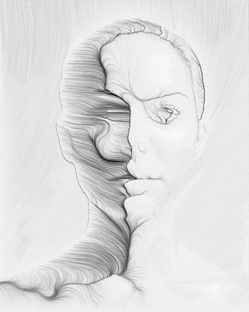
(To be honest I have no idea how to call this organic object).
In this article I describe how to achieve such effect. Generally speaking it’s really simple particle system with also simple attract/repel model based on love/hate attributes. This is step-by-step tutorial.
Particles
Let’s build first our basis – particles. What we need are:
- current position
- current velocity
- age – we want them to die sometimes
- color
- id – to distinguish them
And of course something to init, update and draw. First we draw them on the distorted circle. Behaviour (interactions and movement) will be the next step and will be calculated externally.
// number of particles
final static int N = 500;

// colors (some of them taken from http://www.colourlovers.com/pattern/5526827/bleak
final static color[] cols = { #FF8A00, #FFD200, #749D9D, #FCF5B3, #B39500, #272429 };

// collection of all particles
ArrayList particles = new ArrayList(N);

void setup() {
  size(800,800);
  noFill();
  smooth(8);
  strokeWeight(2.0); // exaggerate a little bit for a while
  background(0,0,20);

  // initialize particles
  for(int i=0;i<N;i++) {
   particles.add( new Particle(i) );
  }
}

void draw() {
  for(Particle p : particles) {
    p.draw();
  }
}

class Particle {
  // position
  float x,y;
  // step
  float dx, dy;
  // id
  int id;
  // life length
  float age;
  // some random color
  color c = cols[(int)random(cols.length)];

  void reset() {
    // distribute initial point on the ring, more near the outer edge, distorted
    float angle = random(TWO_PI);
    float r = 5.0*randomGaussian() + (width/2-100)*(1.0-pow(random(1.0),7.0));
    x = cos(angle)*r;
    y = sin(angle)*r;

    // set random age
    age = (int)random(100,1000);
  }

  void draw() {
   stroke(c);
   point(x+width/2,y+height/2);
  }

  // update position with externally calculated speed
  // check also age
  void update() {
    x += dx;
    y += dy;
    if(--age < 0) reset();
  }

  Particle(int i) {
    id = i;
    reset();
  }
}
Here is the initial result

Behaviour
The most important part, how we move them. Here is the only rule.
For every particle pair: if they love each other attract, reppel otherwise. That’s all.
Ok, detail is: what can be love/hate factor?
Basic love factor
The most obvious is distance. And this one is used here. Formula is

- If distance is larger than 2.0 attract with love amount
- Repel otherwise
Let’s see this.
// number of particles
final static int N = 500;

// colors (some of them taken from http://www.colourlovers.com/pattern/5526827/bleak
final static color[] cols = {
  #FF8A00, #FFD200, #749D9D, #FCF5B3, #B39500, #272429
};

// collection of all particles
ArrayList particles = new ArrayList(N);

void setup() {
  size(800, 800);
  noFill();
  smooth(8);
  strokeWeight(0.7);
  background(0, 0, 20);

  // initialize particles
  for (int i=0; i<N; i++) {
    particles.add( new Particle(i) );
  }
}

void draw() {
  for (Particle p : particles) {

    // love/hate vector
    float lovex = 0.0;
    float lovey = 0.0;

    for (Particle o : particles) {
      // do not compare with yourself
      if (p.id != o.id) {
        // calculate vector to get distance and direction
        PVector v = new PVector(o.x-p.x, o.y-p.y);
        float distance = v.mag();
        float angle = v.heading();

        // love!
        float love = 1.0 / distance;
        // or hate...
        if (distance<2.0) love = -love;

        // not too fast!
        love *= 0.3;

        // update love vector
        lovex += love * cos(angle);
        lovey += love * sin(angle);
      }

      // calculated love vector will be our speed in resultant direction
      p.dx = lovex;
      p.dy = lovey;
    }
  }

  // update and draw
  for (Particle p : particles) {
   p.update();
   p.draw();
  }
}

class Particle {
  // position
  float x, y;
  // velocity
  float dx, dy;
  // id
  int id;
  // life length
  float age;
  // some random color
  color c = cols[(int)random(cols.length)];

  void reset() {
    // distribute initial point on the ring, more near the outer edge, distorted
    float angle = random(TWO_PI);
    float r = 5.0*randomGaussian() + (width/2-100)*(1.0-pow(random(1.0), 7.0));
    x = cos(angle)*r;
    y = sin(angle)*r;

    // set random age
    age = (int)random(100, 1000);
  }

  void draw() {
    stroke(c,50);
    point(x+width/2, y+height/2);
  }

  // update position with externally calculated speed
  // check also age
  void update() {
    x += dx;
    y += dy;
    if (--age < 0) reset();
  }

  Particle(int i) {
    id = i;
    reset();
  }
}

Nice, we have branching and organic look already. Our particles attract mostly, repel only when distance is low.
Attribute love factor
Now let’s introduce another attribute of our particle. It will be nonnegative floating point value . Let’s call it mood. Rule:
Our particles love each other when they have similar mood. Hate otherwise.
That means that we have to calculate similarity factor between moods to get love factor. The similarity should be between 


One note: don’t be strict with similarity factor, some unbalance between love and hate gives different results.
What can be mood?
- inital angle
- noise value from current position and time (mood changes while particle moves and time goes on)
- some vector field
- etc…
The code for second case as follows
// number of particles
final static int N = 500;

// colors (some of them taken from http://www.colourlovers.com/pattern/5526827/bleak
final static color[] cols = {
  #FF8A00, #FFD200, #749D9D, #FCF5B3, #B39500, #272429
};

// collection of all particles
ArrayList particles = new ArrayList(N);

void setup() {
  size(800, 800);
  noFill();
  smooth(8);
  strokeWeight(0.7);
  background(0, 0, 20);

  // initialize particles
  for (int i=0; i<N; i++) {
    particles.add( new Particle(i) );
  }
}

float time = 0.0;
void draw() {
  for (Particle p : particles) {

    // love/hate vector
    float lovex = 0.0;
    float lovey = 0.0;

    for (Particle o : particles) {
      // do not compare with yourself
      if (p.id != o.id) {
        // calculate vector to get distance and direction
        PVector v = new PVector(o.x-p.x, o.y-p.y);
        float distance = v.mag();
        float angle = v.heading();

        // love!
        float love = 1.0 / distance;
        // or hate...
        if (distance<2.0) love = -love;

        // mood factor
        love *= p.moodSimilarity(o);
        // not too fast!
        love *= 0.5;

        // update love vector
        lovex += love * cos(angle);
        lovey += love * sin(angle);
      }

      // calculated love vector will be our speed in resultant direction
      p.dx = lovex;
      p.dy = lovey;
    }
  }

  // update and draw
  for (Particle p : particles) {
    p.update();
    p.draw();
  }

  time += 0.001;
}

class Particle {
  // position
  float x, y;
  // velocity
  float dx, dy;
  // id
  int id;
  // life length
  float age;
  // some random color
  color c = cols[(int)random(cols.length)];

  // mood factor
  float mood;

  void reset() {
    // distribute initial point on the ring, more near the outer edge, distorted
    float angle = random(TWO_PI);
    float r = 5.0*randomGaussian() + (width/2-100)*(1.0-pow(random(1.0), 7.0));
    x = cos(angle)*r;
    y = sin(angle)*r;
    // set random age
    age = (int)random(100, 2000);
    calcMood();
  }

  void draw() {
    stroke(c,50);
    point(x+width/2, y+height/2);
  }

  // update position with externally calculated speed
  // check also age
  void update() {
    if(--age < 0) {
      reset();
    } else {
      x += dx;
      y += dy;
      calcMood();
    }
  }

  Particle(int i) {
    id = i;
    reset();
  }

  // compare moods
  float moodSimilarity(Particle p) {
    return 1.0-abs(p.mood-this.mood);
  }

  // calculate current mood
  private void calcMood() {
    mood = sin(noise(x/10.0,y/10.0,time)*TWO_PI);
  }
 }

What’s next?
You can mess with several factors in this small model, eg:
- number of particles (beware, it’s
)
- particle size, colors, alpha
- dinstance love/hate formulas (eg. hate distance)
- love amount (“not too fast!” comment)
- time speed
- initial position and age
- moodSimilarity and calcMood functions
Here are some examples:


Influences
Here are some links which guided me to this concept:
- http://www.complexification.net/gallery/machines/happyPlace/ – love/hate concept
- http://inconvergent.net/#writing – growth systems
- http://julienleonard.com/tutorials.html – growth systems
- https://ocw.mit.edu/courses/mathematics/18-177-universal-random-structures-in-2d-fall-2015/index.htm – random growth
Left to explore more deeply: random growth guided by vector field.
Enjoy!

UPDATE: Reddit elpepe5 user worked on this topic a little bit and created really nice results. Found the on GITHUB
]]>
In last article I’ve made the research about vector fields and movement based on it. This time I’m going to treat values from noise (and other functions) as acceleration.
Instead of reading an angle from noise and apply step to my drawing agents I’ll be changing angle itself and then use it in drawing step.
The code
This time drawing code looks like this. Marked line is responsible for modification of the angle.
//drawing agent
class Agent {
  PVector pos; // position of the agent
  float angle; // current angle of the agent

  void update() {
    // modify position using current angle
    pos.x += cos(angle);
    pos.y += sin(angle);

    // get point coordinates
    float xx = map(pos.x, 0, width, -1, 1);
    float yy = map(pos.y, 0, height, -1, 1);

    PVector v = new PVector(xx, yy);

    // modify an angle using noise information
    angle += map( noise(v.x, v.y), 0, 1, -1, 1);
  }
}

// all agents in the list
ArrayList<Agent> agents = new ArrayList<Agent>();

void setup() {
  size(800, 800);
  background(240);
  stroke(20, 10);
  smooth(8);
  strokeWeight(0.7);

  // initialize in random positions
  for (int i=0; i<5000; i++) {
    Agent a = new Agent();
    float posx = random(200, 600);
    float posy = random(200, 600);
    a.pos = new PVector(posx, posy);
    a.angle = random(TWO_PI);
    agents.add(a);
  }
}

float time = 0;
void draw() {
  for (Agent a : agents) {
    pushMatrix();
    // position
    translate(a.pos.x, a.pos.y);
    // rotate
    rotate(a.angle);
    // paint
    point(0, 0);
    popMatrix();
    // update
    a.update();
  }
  time += 0.001;
}

Scaling
After scaling and shifting noise I got more interesing patterns.
void update() {
  // modify position using current angle
  pos.x += cos(angle);
  pos.y += sin(angle);

  // get point coordinates
  float xx = 3 * map(pos.x, 0, width, -1, 1);
  float yy = 3 * map(pos.y, 0, height, -1, 1);

  PVector v = new PVector(xx, yy);
  v.add(new PVector(5,-3));

  // modify an angle using noise information
  angle += 3 * map( noise(v.x, v.y), 0, 1, -1, 1);
}


Applying variations
The other results can be achieved by using variations and curves described in previous articles: Folds and Drawing vector field. Just copy them at the end of the file. Change marked line from the previous code for following code for example:
PVector v = swirl(new PVector(xx, yy),1);

Other variations produce different results and patterns.


Or something like this:
float n1 = noise(xx+5,yy-3)-0.55;

PVector vc = kampyle(n1);
PVector v = sinusoidal(vc,1);
v.mult(5);
v.add(new PVector(5,-3));

Time
As previously we can add time to get noise change during drawing. It gives nice, tissue like, objects.
angle += (3+time) * map( noise(v.x, v.y, time), 0, 1, -1, 1);


Forced movement
Another method is to add some constant value to x position in order to force movement of the points towards the right side.
Lets position all points on the left side during initialization and make number of point smaller.
// initialize in random positions
for (int i=0; i<2000; i++) {
  Agent a = new Agent();
  float posx = 100;
  float posy = random(200, 600);
  a.pos = new PVector(posx, posy);
  a.angle = random(TWO_PI);
  agents.add(a);
}
Then force movement
void update() {
  // modify position using current angle
  pos.x += cos(angle)+0.1;
  pos.y += sin(angle);

  // get point coordinates
  float xx = 3 * map(pos.x, 0, width, -1, 1);
  float yy = 3 * map(pos.y, 0, height, -1, 1);

  PVector v = new PVector(xx,yy);
  v.add(new PVector(5,-3));

  // modify an angle using noise information
  angle += (5+time) * map( noise(v.x, v.y), 0, 1, -1, 1);
}

Using some previous techniques (variations and curves) I got also such results


Or something like this.


Play and enjoy 
The end
Questions? [email protected] or Follow @generateme_blog
Blogs:
]]>

The goal
During last few days I’ve made several attempts to create and visualize 2D vector fields. In the following article you can read about this concept with several examples and code in Processing.
There are many beautiful art/code based on vector field visualization around the net. Mostly based on noise function. Check them out before you start:
- Visualizer by p5art
- Furfrolic by Holger Lippmann
- My own two sketches drawing_generative and threadraw
- Few examples on OpenProcessing site: 1, 2, 3, 4
What is the vector field?
Vector field (in our case) is just a
Why vector? Because you can treat a pair of 

Vector fields can be visualised in the following way


How to get the vector field
The main goal, in this article, is to research various ways to create vector fields. There two cases.
We can operate on functions which returns pair of values like variations. In this case such function defines vector field itself. We can use also some vector operations (like substraction, sum, etc…) to get new functions.
The second option is to get single float number 
Drawing method
The method is quite simple.
- Create points from
floating point range
- Draw them
- For each of the point calculate relating vector from the vector field
- Scale it and add to the point coordinates
- Repeat 2-4
Step 4 is key here. We move our points along vectors. Trace lines build the resulting image.
The general flow for constructing vector field follows this scheme:
![p=(x,y)\mapsto [multiple operations]\mapsto \vec{v}](proxy.php?url=https://s0.wp.com/latex.php?latex=p%3D%28x%2Cy%29%5Cmapsto+%5Bmultiple+operations%5D%5Cmapsto+%5Cvec%7Bv%7D&bg=fff&fg=444444&s=0&c=20201002)
Note: I assume that on every step I can multiply function variables or returned values by any number.
Here is code stub for my experiments
// dynamic list with our points, PVector holds position
ArrayList<PVector> points = new ArrayList<PVector>();

// colors used for points
color[] pal = {
  color(0, 91, 197),
  color(0, 180, 252),
  color(23, 249, 255),
  color(223, 147, 0),
  color(248, 190, 0)
};

// global configuration
float vector_scale = 0.01; // vector scaling factor, we want small steps
float time = 0; // time passes by

void setup() {
  size(800, 800);
  strokeWeight(0.66);
  background(0, 5, 25);
  noFill();
  smooth(8);

  // noiseSeed(1111); // sometimes we select one noise field

  // create points from [-3,3] range
  for (float x=-3; x<=3; x+=0.07) {
    for (float y=-3; y<=3; y+=0.07) {
      // create point slightly distorted
      PVector v = new PVector(x+randomGaussian()*0.003, y+randomGaussian()*0.003);
      points.add(v);
    }
  }
}

void draw() {
  int point_idx = 0; // point index
  for (PVector p : points) {
    // map floating point coordinates to screen coordinates
    float xx = map(p.x, -6.5, 6.5, 0, width);
    float yy = map(p.y, -6.5, 6.5, 0, height);

    // select color from palette (index based on noise)
    int cn = (int)(100*pal.length*noise(point_idx))%pal.length;
    stroke(pal[cn], 15);
    point(xx, yy); //draw

    // placeholder for vector field calculations

    // v is vector from the field
    PVector v = new PVector(0, 0);

    p.x += vector_scale * v.x;
    p.y += vector_scale * v.y;

    // go to the next point
    point_idx++;
  }
  time += 0.001;
}

When I change my field vector to be constant one (different than 0), my points start move.
PVector v = new PVector(0.1, 0.1);

Perlin noise
Let’s begin with perlin noise in few configurations. I’m going to change only marked lines from the code stub.
Variant 1
noise(x,y) function in processing returns value from 0 to 1 (actually implementation used in Processing has some problems and real value is often in range from 0.2 to 0.8). I will treat resulted value as an angle in polar coordinates and use sin()/cos() functions to convert it to cartesian ones. To properly do this I have to scale it up to range ![[0,2\pi ]](proxy.php?url=https://s0.wp.com/latex.php?latex=%5B0%2C2%5Cpi+%5D&bg=fff&fg=444444&s=0&c=20201002)
![[-\pi, \pi ]](proxy.php?url=https://s0.wp.com/latex.php?latex=%5B-%5Cpi%2C+%5Cpi+%5D&bg=fff&fg=444444&s=0&c=20201002)
// placeholder for vector field calculations
float n = TWO_PI * noise(p.x,p.y);
PVector v = new PVector(cos(n),sin(n));

Variant 2
Let’s check what happens when I multiply noise by 10, 100, 300 or even 1000. Noise is now scaled to range ![[-1.1]](proxy.php?url=https://s0.wp.com/latex.php?latex=%5B-1.1%5D&bg=fff&fg=444444&s=0&c=20201002)
float n = 10 * map(noise(p.x/5,p.y/5),0,1,-1,1); // 100, 300 or 1000
PVector v = new PVector(cos(n),sin(n));


Variant 3
Two of above variants were using classic method. Now I get rid of polar->cartesian conversion and I’m going to treat returned value from noise() as cartesian coordinates. Angle of the vector is the same for whole field and only length of vector is changed. This leads to some interesting patterns. Experiment with scaling input coordinates and
float n = 5*map(noise(p.x,p.y),0,1,-1,1);
PVector v = new PVector(n,n);


Parametric curves
Let’s use parametric curves to convert noise() result into vector. The big list of them is defined in Wolfram Alpha or named here. Parametric curve (or plane curve) is a function 
Astroid
// placeholder for vector field calculations
float n = 5*map(noise(p.x,p.y),0,1,-1,1); // and 2

float sinn = sin(n);
float cosn = cos(n);

float xt = sq(sinn)*sinn;
float yt = sq(cosn)*cosn;

PVector v = new PVector(xt,yt);
Results for noise scale 2 and 5


Cissoid of Diocles
// placeholder for vector field calculations
float n = 3*map(noise(p.x,p.y),0,1,-1,1);

float sinn2 = 2*sq(sin(n));

float xt = sinn2;
float yt = sinn2*tan(n);

PVector v = new PVector(xt,yt);

Kampyle of Eudoxus
// placeholder for vector field calculations
float n = 6*map(noise(p.x,p.y),0,1,-1,1);

float sec = 1/sin(n);

float xt = sec;
float yt = tan(n)*sec;

PVector v = new PVector(xt,yt);

Rectangular Hyperbola
// placeholder for vector field calculations
float n = 10*map(noise(p.x*2,p.y*2),0,1,-1,1);

float xt = 1/sin(n);
float yt = tan(n);

PVector v = new PVector(xt,yt);

Superformula
// placeholder for vector field calculations
float n = 5*map(noise(p.x,p.y),0,1,-1,1);

float a = 1;
float b = 1;
float m = 6;
float n1 = 1;
float n2 = 7;
float n3 = 8;

float f1 = pow(abs(cos(m*n/4)/a),n2);
float f2 = pow(abs(sin(m*n/4)/b),n3);
float fr = pow(f1+f2,-1/n1);

float xt = cos(n)*fr;
float yt = sin(n)*fr;

PVector v = new PVector(xt,yt);

Noise and curves combined
Now I’m going to play with some combinations of above curves and make multiple passes through noise().
Let’s put all curves into functions (paste following code to the end of the script):
PVector circle(float n) { // polar to cartesian coordinates
  return new PVector(cos(n), sin(n));
}

PVector astroid(float n) {
  float sinn = sin(n);
  float cosn = cos(n);

  float xt = sq(sinn)*sinn;
  float yt = sq(cosn)*cosn;

  return new PVector(xt, yt);
}

PVector cissoid(float n) {
  float sinn2 = 2*sq(sin(n));

  float xt = sinn2;
  float yt = sinn2*tan(n);

  return new PVector(xt, yt);
}

PVector kampyle(float n) {
  float sec = 1/sin(n);

  float xt = sec;
  float yt = tan(n)*sec;

  return new PVector(xt, yt);
}

PVector rect_hyperbola(float n) {
  float sec = 1/sin(n);

  float xt = 1/sin(n);
  float yt = tan(n);

  return new PVector(xt, yt);
}

final static float superformula_a = 1;
final static float superformula_b = 1;
final static float superformula_m = 6;
final static float superformula_n1 = 1;
final static float superformula_n2 = 7;
final static float superformula_n3 = 8;
PVector superformula(float n) {
  float f1 = pow(abs(cos(superformula_m*n/4)/superformula_a), superformula_n2);
  float f2 = pow(abs(sin(superformula_m*n/4)/superformula_b), superformula_n3);
  float fr = pow(f1+f2, -1/superformula_n1);

  float xt = cos(n)*fr;
  float yt = sin(n)*fr;

  return new PVector(xt, yt);
}
Variant 1 – p5art
Code based on p5art web app noisePainting

// placeholder for vector field calculations
float n1 = 10*noise(1+p.x/20, 1+p.y/20); // shift input to avoid symetry
float n2 = 5*noise(n1, n1);
float n3 = 325*map(noise(n2, n2), 0, 1, -1, 1); // 25,325

PVector v = circle(n3);


Variant 2

// placeholder for vector field calculations
float n1 = 15*map(noise(1+p.x/20, 1+p.y/20),0,1,-1,1);

PVector v1 = cissoid(n1);
PVector v2 = astroid(n1);

float n2a = 5*noise(v1.x,v2.y);
float n2b = 5*noise(v2.x,v1.y);

float n3 = 10*map(noise(n2a, n2b/3), 0, 1, -1, 1);

PVector v = circle(n3);

Variant 3

// placeholder for vector field calculations
float n1 = 15*map(noise(1+p.x/10, 1+p.y/10),0,1,-1,1);

PVector v1 = rect_hyperbola(n1);
PVector v2 = astroid(n1);

float n2a = 2*map(noise(v1.x,v1.y),0,1,-1,1);
float n2b = 2*map(noise(v2.x,v2.y),0,1,-1,1);

PVector v = new PVector(n2a,n2b);

Variant 4

// placeholder for vector field calculations
PVector v1 = kampyle(p.x);
PVector v2 = superformula(p.y);

float n2a = 3*map(noise(v1.x,v1.y),0,1,-1,1);
float n2b = 3*map(noise(v2.x,v2.y),0,1,-1,1);

PVector v = new PVector(cos(n2a),sin(n2b));

Variant 5

// placeholder for vector field calculations
float n1a = 3*map(noise(p.x,p.y),0,1,-1,1);
float n1b = 3*map(noise(p.y,p.x),0,1,-1,1);

PVector v1 = rect_hyperbola(n1a);
PVector v2 = astroid(n1b);

float n2a = 3*map(noise(v1.x,v1.y),0,1,-1,1);
float n2b = 3*map(noise(v2.x,v2.y),0,1,-1,1);

PVector v = new PVector(cos(n2a),sin(n2b));

Variant 6 – comparison
Here I want to compare different curves using the same method. I change marked lines into pair of curves defined above. I’ve put noiseSeed(1111); in setup() to have the same noise structure. Check image description to see what curves were used.

// placeholder for vector field calculations
float n1a = 15*map(noise(p.x/10,p.y/10),0,1,-1,1);
float n1b = 15*map(noise(p.y/10,p.x/10),0,1,-1,1);

PVector v1 = superformula(n1a);
PVector v2 = circle(n1b);

PVector diff = PVector.sub(v2,v1);
diff.mult(0.3);

PVector v = new PVector(diff.x,diff.y);


Time
Now let’s introduce time. An external variable which is incremented every frame with some small value. It can be used to slightly change noise field during rendrering or can be used as a scale factor.
Let’s compare the same vector field without time and time used as third noise parameter.
 // placeholder for vector field calculations
 float n1a = 3*map(noise(p.x/2,p.y/2),0,1,-1,1);
 float n1b = 3*map(noise(p.y/2,p.x/2),0,1,-1,1);
 float nn = 6*map(noise(n1a,n1b),0,1,-1,1);

 PVector v = circle(nn);

And now I add time as a third parameter to noise function. This way our vector field changes when time passes.
 // placeholder for vector field calculations
float n1a = 3*map(noise(p.x/2,p.y/2,time),0,1,-1,1);
float n1b = 3*map(noise(p.y/2,p.x/2,time),0,1,-1,1);
float nn = 6*map(noise(n1a,n1b,time),0,1,-1,1);

PVector v = circle(nn);

Now time is used as a scaling factor.
// placeholder for vector field calculations
float n1a = 3*map(noise(p.x/2,p.y/2),0,1,-1,1);
float n1b = 3*map(noise(p.y/2,p.x/2),0,1,-1,1);

float nn = time*10*6*map(noise(n1a,n1b),0,1,-1,1);

PVector v = circle(nn);

Variations
Now let’s introduce variations (see previous post about Folds) as a vector field definition.
Copy below code to the end of your sketch. It includes function definiotions used in this and next chapters.
PVector sinusoidal(PVector v, float amount) {
  return new PVector(amount * sin(v.x), amount * sin(v.y));
}

PVector waves2(PVector p, float weight) {
  float x = weight * (p.x + 0.9 * sin(p.y * 4));
  float y = weight * (p.y + 0.5 * sin(p.x * 5.555));
  return new PVector(x, y);
}

PVector polar(PVector p, float weight) {
  float r = p.mag();
  float theta = atan2(p.x, p.y);
  float x = theta / PI;
  float y = r - 2.0;
  return new PVector(weight * x, weight * y);
}

PVector swirl(PVector p, float weight) {
  float r2 = sq(p.x)+sq(p.y);
  float sinr = sin(r2);
  float cosr = cos(r2);
  float newX = 0.8 * (sinr * p.x - cosr * p.y);
  float newY = 0.8 * (cosr * p.y + sinr * p.y);
  return new PVector(weight * newX, weight * newY);
}

PVector hyperbolic(PVector v, float amount) {
  float r = v.mag() + 1.0e-10;
  float theta = atan2(v.x, v.y);
  float x = amount * sin(theta) / r;
  float y = amount * cos(theta) * r;
  return new PVector(x, y);
}

PVector power(PVector p, float weight) {
  float theta = atan2(p.y, p.x);
  float sinr = sin(theta);
  float cosr = cos(theta);
  float pow = weight * pow(p.mag(), sinr);
  return new PVector(pow * cosr, pow * sinr);
}

PVector cosine(PVector p, float weight) {
  float pix = p.x * PI;
  float x = weight * 0.8 * cos(pix) * cosh(p.y);
  float y = -weight * 0.8 * sin(pix) * sinh(p.y);
  return new PVector(x, y);
}

PVector cross(PVector p, float weight) {
  float r = sqrt(1.0 / (sq(sq(p.x)-sq(p.y)))+1.0e-10);
  return new PVector(weight * 0.8 * p.x * r, weight * 0.8 * p.y * r);
}

PVector vexp(PVector p, float weight) {
  float r = weight * exp(p.x);
  return new PVector(r * cos(p.y), r * sin(p.y));
}

// parametrization P={pdj_a,pdj_b,pdj_c,pdj_d}
float pdj_a = 0.1;
float pdj_b = 1.9;
float pdj_c = -0.8;
float pdj_d = -1.2;
PVector pdj(PVector v, float amount) {
  return new PVector( amount * (sin(pdj_a * v.y) - cos(pdj_b * v.x)),
  amount * (sin(pdj_c * v.x) - cos(pdj_d * v.y)));
}

final float cosh(float x) { return 0.5 * (exp(x) + exp(-x));}
final float sinh(float x) { return 0.5 * (exp(x) - exp(-x));}
Let’s see how individual variations look as vector fields. Sometimes I had to adjust scaling factor to keep points on the screen.
// placeholder for vector field calculations
PVector v = sinusoidal(p,1);
v.mult(1); // different values for different functions


All together
Let’s sumarize what functions we have now defined.
- multiplying/dividing by number
- single variable noise()
- other single variable functions (sin/cos, exp, log, sq, sqrt, etc.)
- parametric curves
- noise() with two parameters
- distance between vectors
- dot product of vectors
- length of the vector
- angle between vectors
- variations and their combinations
- sum or difference of vectors
- atan2() of the vector


All above operations can be used to generate vector field (or simply transform 2d point to another 2d point).
I will play with above transformations in following examples. It’s a record of experiments.
Variant 1

// placeholder for vector field calculations
float n1 = 5*map(noise(p.x/5,p.y/5),0,1,-1,1);

PVector v1 = rect_hyperbola(n1);
PVector v2 = swirl(v1,1);

PVector v = new PVector(cos(v2.x),sin(v2.y));

Variant 2

// placeholder for vector field calculations
float n1 = 5*map(noise(p.x/5,p.y/5),0,1,-1,1);
float n2 = 5*map(noise(p.y/5,p.x/5),0,1,-1,1);

PVector v1 = vexp(new PVector(n1,n2),1);
PVector v2 = swirl(new PVector(n2,n1),1);

PVector v3 = PVector.sub(v2,v1);

PVector v4 = waves2(v1,1);
v4.mult(0.8);

PVector v = new PVector(v4.x,v4.y);

Variant 3

// placeholder for vector field calculations
PVector v1 = vexp(p,1);

float n1 = map(noise(v1.x,v1.y,time),0,1,-1,1);
float n2 = map(noise(v1.y,v1.x,-time),0,1,-1,1);

PVector v2 = vexp(new PVector(n1,n2),1);

PVector v = new PVector(v2.x,v2.y);

Variant 4

// placeholder for vector field calculations
PVector v1 = polar(cross(p,1),1);

float n1 = 15*map(noise(v1.x,v1.y,time),0,1,-1,1);
PVector v2 = cissoid(n1);
v2.normalize();

PVector v = new PVector(v2.x,v2.y);

Variant 5

// placeholder for vector field calculations
PVector v1 = power(p,1);

float n1 = 5*map(noise(v1.x,v1.y,time),0,1,-1,1);
float n2 = 5*map(noise(p.x/3,p.y/3,-time),0,1,-1,1);

PVector v2 = cosine(new PVector(n1,n2),1);

float a1 = PVector.angleBetween(v1,v2);

PVector v3 = superformula(a1);
v3.mult(3);

PVector v = new PVector(cos(v3.x),sin(v3.y));

Variant 6

// placeholder for vector field calculations
PVector v1 = waves2(p,1);
PVector v2 = PVector.sub(v1,p);

float n1 = 8*noise(time)*atan2(v1.y,v1.x);
float n2 = 8*noise(time+0.5)*atan2(v2.y,v2.x);

PVector v = new PVector(cos(v2.x*n1),sin(v1.y+n2));

Variant 7

// placeholder for vector field calculations
PVector v1 = swirl(p,1);
v1.mult(0.5);
PVector v2 = PVector.sub(v1,p);

float nv1 = noise(v1.x,v1.y,time);
float nv2 = noise(v2.x,v2.y,-time);

float n1 = (atan2(v1.y,v1.x)+nv2);
float n2 = (atan2(v2.y,v2.x)+nv1);

PVector v3 = superformula(n1);
PVector v4 = rect_hyperbola(n2);

PVector tv3 = waves2(v3,1);
PVector tv4 = sinusoidal(v4,1);

PVector v5 = PVector.sub(tv4,tv3);

PVector v6 = pdj(v5,1);

float an = PVector.angleBetween(v6,new PVector(n1,n2));

PVector v = new PVector(cos(v2.x+sin(an)),sin(v6.y-cos(an)));
v.mult(1+time*40);

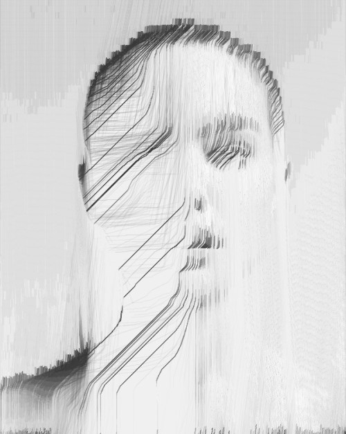
Image
The last part is about using channel information from an image as a vector field. I wrote two sketches some time ago which are based on vector field concept.
Drawing generative
Threadraw
How to use image data
First load your image at the beginning of the sketch
img = loadImage("natalie.jpg"); // PImage img; must be declared globally
Then use image data following way
// placeholder for vector field calculations
PVector v1 = sinusoidal(p,1);

int img_x = (int)map(p.x,-3,3,0,img.width);
int img_y = (int)map(p.y,-3,3,0,img.height);

float b = brightness( img.get(img_x,img_y) )/255.0;
PVector br = circle(b);

float a = 5*PVector.angleBetween(br,v1);

PVector v = astroid(a);

Appendix
This concept is taken from zach lieberman and Keith Peters who explored painting by non-intersecting segments. This idea can be used on vector fields too. Here are two examples.


See the code HERE.
The end
Questions? [email protected] or Follow @generateme_blog
]]>
A few years ago I started to explore fractal flames which resulted in Scratch implementation of flame explorer (https://scratch.mit.edu/projects/17114670/). Click HERE to read about what a fractal flame actually is.
Actually most of the ‘flavour’ in fractal flames is made of something authors call ‘variations’. Variations are nothing more than real number functions from
I’ve started to draw them in a lot of different ways in order to explore their beauty. Here is how I do it:
Variations
A Variation is a multivariable real number function with domain and codomain R^n. I will focus on the 2D version. Sometimes it can have a name map or a morphism, but I call it just a function. So our function converts a point 

Usually a Variation is designed as a whole class of functions, which means there are a few external parameters that you need to set to certain values in order to get a specific function. In such a case a different set of parameters will result in a different function.
The other parameter used is the ‘amount’ of the function. ‘amount’ is a special parameter which in almost all cases scales the resulting value.
So a more formal definition of our function is:
, where
; which means:
Variation V is a function with some sequence of parameters Ρ which is scaled by a factor α. Sequence of parameters Ρ is just a sequence of values which are used in definition of the function.
Although the domain is the whole R² space I usually only operate on [-3,3]x[-3,3] range.
Examples of Variations
Here are some basic ones (without parameters and with α=1):
- Identity –
- Linear –
- Sinusoidal –


Things get more complicated when we add sequence of parameters (and α=1). These definitions are function class definitions and by using specific parameters you will obtain unique functions.
- PDJ –
, where
from
.
, where
- Rectangles –
, where
from
, where


How to draw it
Here is the template I use to draw. The general concept is to take every point from the [-3,3]x[-3,3] range, calculate the result of the function and draw it. This template draws a simple identity function:
void setup() {
  size(600, 600);
  background(250);
  smooth(8);
  noFill();
  stroke(20, 15);
  strokeWeight(0.9);

  x1=y1=-3;
  x2=y2=3;
  y=y1;
  step=(x2-x1)/(2.321*width);
}

float x1, y1, x2, y2; // function domain
float step; // step within domain
float y;

boolean go = true;
void draw() {
  if (go) {
    for (int i=0; (i<20)&go; i++) { // draw 20 lines at once
      for (float x=x1; x<=x2; x+=step) {
        drawVariation(x, y);
      }
      y+=step;
      if (y>y2) {
        go = false;
        println("done");
      }
    }
  }
}

void drawVariation(float x, float y) {
  float xx = map(x, x1, x2, 20, width-20);
  float yy = map(y, y1, y2, 20, height-20);
  point(xx, yy);
}

The result, which you can see here, is a grid that’s the result of rounding floating point values. By inserting the randomGaussian() function into the calculation I can distort the points a little and thus get a less rigid and more uniform look.
void drawVariation(float x, float y) {
  float xx = map(x+0.003*randomGaussian(), x1, x2, 20, width-20);
  float yy = map(y+0.003*randomGaussian(), y1, y2, 20, height-20);
  point(xx, yy);
}

Ok, now we are ready to plot our first functions!
Sinusoidal
Let’s start with a sinusoidal function.
V(x,y) = (αsin(x),αsin(y));
The code to draw this function looks like this:
void drawVariation(float x, float y) {
  PVector v = new PVector(x,y);
  float amount = 1.0;

  v = sinusoidal(v,amount);

  float xx = map(v.x+0.003*randomGaussian(), x1, x2, 20, width-20);
  float yy = map(v.y+0.003*randomGaussian(), y1, y2, 20, height-20);
  point(xx, yy);
}

PVector sinusoidal(PVector v, float amount) {
  return new PVector(amount * sin(v.x), amount * sin(v.y));
}
The top image is a plot with amount=1.0. The bottom image is an example where I used amount=3.0 to scale the resulting value up to the [-3,3]x[-3,3] range.


Hyperbolic
Another example is the hyperbolic function, which uses polar coordinates to calculate x and y.
PVector hyperbolic(PVector v, float amount) {
  float r = v.mag() + 1.0e-10;
  float theta = atan2(v.x, v.y);
  float x = amount * sin(theta) / r;
  float y = amount * cos(theta) * r;
  return new PVector(x, y);
}

PDJ
Now let’s draw functions from the PDJ class. The sequence of parameters are provided as external variables and used in the function.
// parametrization P={pdj_a,pdj_b,pdj_c,pdj_d}
float pdj_a = 0.1;
float pdj_b = 1.9;
float pdj_c = -0.8;
float pdj_d = -1.2;
PVector pdj(PVector v, float amount) {
  return new PVector( amount * (sin(pdj_a * v.y) - cos(pdj_b * v.x)),
                      amount * (sin(pdj_c * v.x) - cos(pdj_d * v.y)));
}
So, for example, when I set Ρ = {0.1, 1.9, -0.8, -1.2} I get:

But with Ρ={1.0111, -1.011, 2.08, 10.2} I get something very different:

See also Holger Lippmann’s works based on PDJ functions
Julia
The next function I want to show is Julia where random() function is used.
PVector julia(PVector v, float amount) {
  float r = amount * sqrt(v.mag());
  float theta = 0.5 * atan2(v.x, v.y) + (int)(2.0 * random(0, 1)) * PI;
  float x = r * cos(theta);
  float y = r * sin(theta);
  return new PVector(x, y);
}

Sech
And then there’s the last function, Sech, which is based on an hyperbolic functions:
float cosh(float x) { return 0.5 * (exp(x) + exp(-x));}
float sinh(float x) { return 0.5 * (exp(x) - exp(-x));}

PVector sech(PVector p, float weight) {
  float d = cos(2.0*p.y) + cosh(2.0*p.x);
  if (d != 0)
    d = weight * 2.0 / d;
  return new PVector(d * cos(p.y) * cosh(p.x), -d * sin(p.y) * sinh(p.x));
}

More to see
Click HERE to see the animations of 129 basic variations that I have created in Scratch
Now let’s complicate things!
Being aware now of the base functions (which are widely available: flame.pdf paper defines 48 of them, JWildfire code defines 200+ usable functions or classes of functions), we can then create new ones ourselves. Math theories (like group/ring theories, homomorphism, analysis, etc) with associativity and distributivity of operations give us recipes to build new functions from the others.
Let’s suppose we have variations 

- Sum of the function:
- Subtraction of the functions:
- Combination of the function:
- Kind of differencial/derivative (it’s not strict differential):
, where
and
is some real number and
- Multiplication:
- Division:
, where when denominator is 0, value is also 0 (just to simplify things)
- Power:
or as recursive combinations:


You can of course mix all of the above to create a bunch of new and unique functions. For example, you can create function which is a sum of combination of power of division of few base functions. Or whatever else you want.
The sum, subtraction, multiplication and division of functions can be coded like this:
PVector addF(PVector v1, PVector v2) { return new PVector(v1.x+v2.x, v1.y+v2.y); }
PVector subF(PVector v1, PVector v2) { return new PVector(v1.x-v2.x, v1.y-v2.y); }
PVector mulF(PVector v1, PVector v2) { return new PVector(v1.x*v2.x, v1.y*v2.y); }
PVector divF(PVector v1, PVector v2) { return new PVector(v2.x==0?0:v1.x/v2.x, v2.y==0?0:v1.y/v2.y); }
Combination can be obtained like this (julia o sech)
v = julia(sech(v,amount),amount);
Power, which is multiple combination of the same function, can be coded like this (hyperbolic^5 = hyperbolic(hyperbolic(hyperbolic(hyperbolic(hyperbolic)))) )
for(int i=0;i<5;i++) v = hyperbolic(v,amount);
And an example of a differential of pdj function:
PVector d_pdj(PVector v, float amount) {
  float h = 0.1; // step
  float sqrth = sqrt(h);
  PVector v1 = pdj(v, amount);
  PVector v2 = pdj(new PVector(v.x+h, v.y+h), amount);
  return new PVector( (v2.x-v1.x)/sqrth, (v2.y-v1.y)/sqrth );
}
hyperbolic + pdj
v = addF( hyperbolic(v,amount), pdj(v,amount) );

julia – hyperbolic
v = subF( julia(v,amount), hyperbolic(v,amount) );

sech * pdj
v = mulF( sech(v,amount), pdj(v,amount) );

hyperbolic / sech
v = divF( hyperbolic(v,amount), sech(v,amount) );

d(pdj)
  float amount = 3.0; // scale up
  v = d_pdj(v,amount);

julia o hyperbolic = julia(hyperbolic)
v = julia(hyperbolic(v,amount),amount);

hyperbolic ^ 10
for(int i=0;i<10;i++) v = hyperbolic(v,amount);

[julia((hyperbolic + julia o sech) * pdj) – d(pdj)]^3
  for(int i=0;i<3;i++)
    v = subF(julia( mulF(addF(hyperbolic(v,0.5),julia(sech(v,1),0.5)),pdj(v,1)),2.5),d_pdj(v,1));

Folding
In the above examples you can see that some of the points have escaped outside of the screen. The main reason is that the values exceeded -3 or 3. To keep them inside our area we have to force them to be in the required range of values. There are a couple of strategies for achieving this. I will describe two of them: modulo and sinusoidal.
I will use pdj + hyperbolic * sech function with amount = 2
  float amount = 2.0;
  v = addF(pdj(v,amount),mulF(hyperbolic(v,amount),sech(v,amount)));
Modulo
The first strategy is to treat the screen as a torus (points that exceed the screen area will reappar on the opposite side: top <> down, left <> right). The formula for this wrapping is documented below. It is called after the function has been calculated.
  v.x = (v.x - x1) % (x2-x1);
  if(v.x<0) v.x += (x2-x1);
  v.y = (v.y - y1) % (y2-y1);
  if(v.y<0) v.y += (y2-y1);
  v.x += x1;
  v.y += y1;

Sinusoidal
The second strategy is to wrap the points using a sinus function, which moves between -1 to 1. With amount=3 you get the required range.
v = sinusoidal(v,(x2-x1)/2);

Towards fixed point
In maths a ‘fixed point’ is a special point a where f(a) = a. If the function has a special characteristic (is a contraction mapping) a fixed point can be calculated by using the power of the function as defined above. Just call f(f(f(f(f(f….))))). In our case we operate on a set of points (range [-3,3]x[-3,3]) and our “fixed point” can also be set (if exists). So let’s try to modify our code a little and draw each step for a certain power of our function.
Let’s create a function v = sinusoidal o julia o sech calculate v(v(v(v(…)))) and draw each step: first v, then v(v), v(v(v)), in order to finish at some chosen number.
Our algorithm will look like this:
- set n = 3
- choose a point p = (x,y)
- calculate new point p = sinusoidal(julia(sech(p)))
- draw point p
- repeat n (=3) times steps 3-4 (using newly calculated point p)
- go to 2
But first we need to adjust the step value and set the stroke color to be slightly lighter
  stroke(60, 15);
  //...
  // more points drawn in drawVariation, bigger step
  step=sqrt(n)*(x2-x1)/(2.321*width);
And adapt drawVariation()
int n=1;
void drawVariation(float x, float y) {
  PVector v = new PVector(x, y);

  for (int i=0; i<n; i++) {
    v = julia(sech(v, 1), 1);
    v = sinusoidal(v, (x2-x1)/2);
    float xx = map(v.x+0.003*randomGaussian(), x1, x2, 20, width-20);
    float yy = map(v.y+0.003*randomGaussian(), y1, y2, 20, height-20);
    point(xx, yy);
  }
}
The following images represent represent values of n = 1, 2, 4, 8, 16, 32, 64, 128.


For high n the sequence will finally result in this (it’s a fixed point of our function)

Folds2d
To produce my works I prepared a few more things to have more variety of functions and semi-artistic look. These are:
- JWildfire wrapper for Processing (to get all Variations included there)
- Random formula generator with evaluation
- Randomization of parameters
- Noisy, gray canvas
- High resolution rendering
- Fixed point option
- Scaling / translating range
- Various folding options
- and probably few more
Final notes
I would like to THANK Jerome Herr for review of this article. Thank you very much man!
Don’t forget to visit his page: http://p5art.tumblr.com/
Questions/Errors? [email protected]

]]>
Ok, so, you’re bored, have spare time, have working caffe on gpu and want to try train network to get rid of dogs in deep dream images… Here is tutorial for you. In points.
- Forget about training from the scratch, only fine tune on googlenet. Building net from the scratch requires time, a lot of time, hundreds of hours… Read it first: http://caffe.berkeleyvision.org/gathered/examples/finetune_flickr_style.html.
- The hardest part: download 200-1000 images you want to use for training. I found that one type of images work well. Faces, porn, letters, animals, guns, etc.
- Resize all images into dimension of 256×256. Save it as truecolor jpgs (not grayscale, even if they are grayscale)
- OPTION: Calculate average color values of all your images. You need to know what is average value of red, green and blue of your set. I use command line tools convert and identify from ImageMagick: convert *.jpg -average res.png; identify -verbose res.png to see ‘mean’ for every channel.
- Create folder <caffe_path>/models/MYNET <- this will be your working folder. All folders and files you’ll create will be placed in MYNET
- Create folder named ‘images’ (in your working folder, MYNET)
- For every image you have create separate folder in ‘images’. I use numbers starting from 0. For example ‘images/0/firstimage.jpg’, ‘images/1/secondimage.jpg’, etc… Every folder is a category. So you end up with several folders with single image inside.
- Create text file called train.txt (and put it to the working folder). Every line of this file should be relative path of the image with the number of the image category. It looks like this:
images/0/firstimage.jpg 0
images/1/secondimage.jpg 1
… - Copy train.txt into val.txt file
- Copy deploy.prototxt, train_val.prototxt and solver.prototxt into working folder from this link: https://gist.github.com/tsulej/ff2b3e37aa76e8fbb244
- Next you need to edit all files, let’s start.
- train_val.prototxt:
- lines 13-15 (and 34-36) define mean values for your image set. For blue, green and red channels respectively (mind the reverse order). If you don’t know them just set all to 129
- line 19, define number of images processed at once. 40 works well on 4gb GPU. You need probably change it to 20 for 2gb gpu. You’ll get out of memory error if number is too high, then just lower it. You can set it to 1 as well.
- lines 917, 1680 and 2393. num_output should be set to number of your categories (number of your folders in image folder)
- deploy.prototxt:
- line 2141, num_output as above
- solver.prototxt, what is important below:
- display: 20 – print statistics every 20 iterations
- base_lr: 0.0005 – learning rate, it’s a subject to change. You’ll be observing loss value and adapt base_lr regarding results (see strategy below)
- max_iter: 200000 – how many iterations for training, you can put here even million.
- snapshot: 5000 – how often create snapshot and network file (here, every 5000 iterations). It’s important if you want to break training in the middle.
- Almost ready to train… but you need googlenet yet. Go to caffe/models/bvlc_googlenet and download this file (save it here) http://dl.caffe.berkeleyvision.org/bvlc_googlenet.caffemodel
- Really ready to train. Go to the working folder and run this command:
../../build/tools/caffe train -solver ./solver.prototxt -weights ../bvlc_googlenet/bvlc_googlenet.caffemodel
It should work. Every 5000 iterations you’ll get snapshot. You can break training then and run deepdream on your net. First results should be visible on inception_5b/output layer.
To restart training use a snapshot running this command:
../../build/tools/caffe train -solver ./solver.prototxt -snapshot ./MYNET_iter_5000.solverstate
Strategy for base_lr in solver for first 1000 iterations. Observe loss value. During the training it should be in average lower and lower and go towards 0.0. But:
- if you see ‘loss’ value during training is higher and higher – break and set base_lr 5 times less than current
- if you see ‘loss’ stuck at near some value and lowers but very slowly – break and set base_lr 5 times more than current
- if none of above strategy works – probably you have troubles and train failed. Change image set and start over.
Some insights:
- My GPU is NVIDIA GTX960 with 4gb RAM. Caffe is compiled with CuDNN library. Every 5k iterations take about 1 hour. On CPU calculations were 40 times slower.
- I usually stop after 40k of iterations. But did also 90k. DeepDickDream guy made 750k iterations to have dicks on Hulk Hogan (http://deepdickdreams.tumblr.com/)
- You have little chance to get your image set visible in deepdreams images before 100k of iterations. But you have high probability to see something new and no dogs
- Fine tune method means that you copy almost all information into your net from existing net except the layers called “classification” (three of them). To achieve this just rename layer name. You may decide and try not to copy other layers (eg. all inception_5b) to clean up more information. I have good and bad results using this method. To do this just change name of such layer.
- You can put more images into one category. You can use 20 categories with 200 images in it. You can use random images, same images, similar images, whatever you want. I couldn’t find a rule to get best results. It depends mostly on content I suppose.
Examples:
Net trained on british library images (https://www.flickr.com/photos/britishlibrary/albums ). 11 categories. 100k images total (every image had 10 variants). inception layer 3, 4 and 5 were cleaned up. Result after 25k iterations. Faces from portrait album are clearly visible. This was my first and best try (among 20). Image from 5b/output layer.

Only letters album from british library images. 750 categories with one image in category. 40k iteration. Only classification layers cleaned up. Butterflies visible, but why? Layer 5b.

Same as above. 5a layer. Hourglasses. 
94 categories, 100 images each, porn image set. 90k iterations. default net set (only classification). Layer 5b. 
As above but differently prepared image set (flip/flop, rotations, normalization/equalization, blur/unsharp, etc.). 40k iterations. Layer 5b. 
Caffenet, built from scratch on 4 categories, 1000 glitch images each. 65k iterations. Pool5 layer. 
Same image set as above. 80k iterations. googlenet with cleaned up 3, 4 and 5 layers. 5b layer. 
Any questions? Comment it or write [email protected]
]]>

Wool
I’ll try to recreate process from the scratch showing ready-to-use code progressively.
Inspiration
In addition to my own, a lot of ideas are taken from others’ works. It can be a specific palette, technique, composition, structure or texture. Then I recreate, rework, inspire myself by them to build my own dictionary and toolset. Still learning and searching.
This time it was picture by SuperColony:

217/365 by SuperColony
Fortunately guys published source code and it was beginning for me.
Analysis
Code is quite simple and easy to understand but the result isn’t obvious. Let’s simplify code a little and draw one step.

void setup() {
  size(800,800);
  smooth(8);
  noFill();
  stroke(233, 131, 45);
  makeme();
}

float yoff = 0.0;
void makeme() {
  background(23, 67, 88);
  strokeWeight(2*noise(20,200));
  beginShape();
  float xoff2 = 0;
  for (float x = 0; x <= width; x += 5) {
    float y = map(noise(xoff2, yoff*20), 0, 1, 20, 800);
    vertex(x, y);
    xoff2 += random(0.01,0.05);
  }
  yoff += 0.01;
  vertex(width, height);
  vertex(0, height);
  endShape(CLOSE);
}

void draw() {}
void keyPressed() { saveFrame("f####.png"); }
void mousePressed() { makeme(); }
So, this is simply plot of noise function (line 16) using vertex(). If we draw 2000 steps we’ll see expected result. Originally authors chose 2 different colors (with alpha ranging from 5 to 20) and 3 positions of plot sets.

void setup() {
  size(800,800);
  smooth(8);
  noFill();
  makeme();
}

float yoff = 0.0;
void makeme() {
  background(23, 67, 88);
  for(int iter=0;iter<2000;iter++) {
    stroke(233, 131, 45, random(5,20));
    strokeWeight(2*noise(20,200));
    beginShape();
    float xoff2 = 0;
    for (float x = 0; x <= width; x += 5) {
      float y = map(noise(xoff2, yoff*20.0), 0, 1, 20, 800);
      vertex(x, y);
      xoff2 += random(0.01,0.05);
    }
    yoff += 0.01;
    vertex(width, height);
    vertex(0, height);
    endShape(CLOSE);
  }
}

void draw() {}
void keyPressed() { saveFrame("f####.png"); }
void mousePressed() { makeme(); }
Our picture represents traverse of noise field with almost the same x range (lines 15 and 19) and different y each line. We can see that we have some kind of periodicity. It leads to the conclusion that noise function is periodic. And this characteristic makes the effect. If you change line 15th to have xoff2 initialized randomly you can bypass this issue.
float xoff2 = random(1.0);

Ok. This is enough to start with my own version.
Step 1 – Circle
Let’s make a circle from above wool-a-like structure, reset colors (will be decided later). To make circle just switch to polar coordinates. Random some attributes (xoff, yoff, ang step) to avoid regularity. Unfortunately nasty thing happens at angle=0.0. It’s due to fact that lines doesn’t join at the same point, traversing noise field I don’t return to the starting position.

void setup() {
  size(800,800);
  smooth(8);
  noFill();
  makeme();
}

float yoff = random(1.0);
void makeme() {
  background(20);
  translate(400,400);
  for(int iter=0;iter<3000;iter++) {
    stroke(240, random(5.0,20.0));
    strokeWeight(random(1.0));
    float xoff = random(1.0);
    beginShape();
    for (float ang=0.0; ang<TWO_PI; ang+=random(TWO_PI/200.0)) {
      float r = map(noise(xoff, yoff*5.0), 0, 1, 20, 400);
      float x = r * cos(ang);
      float y = r * sin(ang);
      vertex(x, y);
      xoff += random(0.01,0.05);
    }
    yoff += random(0.01,0.05);
    endShape(CLOSE);
  }
}

void draw() {}
void keyPressed() { saveFrame("f####.jpg"); }
void mousePressed() { makeme(); }
Step 2 – Break the circle
To bypass this issue just make the gap wider. To make it change line 17. Better but sharp edges are not so pleasant.

for (float ang=0.0; ang<0.8*TWO_PI; ang+=random(TWO_PI/200.0)) {
Step 3 – Adjustment
To fix it let’s random a little beginning and end of the arc. And provide variable shape_closed to make two options: one with closed circle and other with open.


void setup() {
  size(800,800);
  smooth(8);
  noFill();
  makeme();
}

void makeOptions() {
  shape_closed = random(1)<0.5 ? true : false;
}

boolean shape_closed = true;
float yoff = random(1.0);
void makeme() {
  background(20);
  translate(400,400);
  makeOptions(); // calculate some random parameters
  for(int iter=0;iter<3000;iter++) {
    stroke(240, random(5.0,20.0));
    strokeWeight(random(1.0));
    float xoff = random(1.0);
    beginShape();
    for (float ang=random(0.2); ang<random(0.8,0.9)*TWO_PI; ang+=random(TWO_PI/200.0)) {
      float r = map(noise(xoff, yoff*5.0), 0, 1, 20, 400);
      float x = r * cos(ang);
      float y = r * sin(ang);
      vertex(x, y);
      xoff += random(0.01,0.05);
    }
    yoff += random(0.01,0.05);
    if(shape_closed) endShape(CLOSE); else endShape();
  }
}

void draw() {}
void keyPressed() { saveFrame("f####.jpg"); }
void mousePressed() { makeme(); }
Step 4 – Shift
This time let’s shift and make some distance of two halves. Make it optional (choosen randomly).


void setup() {
  size(800,800);
  smooth(8);
  noFill();
  makeme();
}

void makeOptions() {
  shape_closed = random(1)<0.5 ? true : false;
  shiftxy = (int)random(3);
}

int shiftxy = 0;
boolean shape_closed = true;
float yoff = random(1.0);
void makeme() {
  background(20);
  translate(400,400);
  makeOptions(); // calculate some random parameters
  for(int iter=0;iter<3000;iter++) {
    stroke(240, random(5.0,20.0));
    strokeWeight(random(1.0));
    float xoff = random(1.0);
    beginShape();
    for (float ang=random(0.2); ang<random(0.8,0.9)*TWO_PI; ang+=random(TWO_PI/200.0)) {
      float r = map(noise(xoff, yoff*5.0), 0, 1, 20, 400);
      float x = r * cos(ang);
      float y = r * sin(ang);

      if( (shiftxy == 1 && x>0.0) || (shiftxy == 2 && y>0.0)) {
        x += 20.0;
        y += 20.0;
      } else if(shiftxy > 0.0) {
        x -= 20.0;
        y -= 20.0;
      }

      vertex(x, y);
      xoff += random(0.01,0.05);
    }
    yoff += random(0.01,0.05);
    if(shape_closed) endShape(CLOSE); else endShape();
  }
}

void draw() {}
void keyPressed() { saveFrame("f####.jpg"); }
void mousePressed() { makeme(); }
Step 5 – Blocks
I like rectangular view or similar distortions so here I going to divide my picture to squares and inside each square exchange x and y axises. Of course let’s make it optional. Calculating abs() of x or y (line 46 and 47) stops exchanging x/y for negative values. One more issue: when doing blocks all points are moved by square size we need to adjust it (line 25)


void setup() {
  size(800,800);
  smooth(8);
  noFill();
  makeme();
}

void makeOptions() {
  shape_closed = random(1)<0.5 ? true : false;
  shiftxy = (int)random(3);
  do_absx = random(1)<0.5 ? true : false;
  do_absy = random(1)<0.5 ? true : false;
  do_blocky = random(1)<0.75 ? true : false;
}

boolean do_absx=false;
boolean do_absy=false;
boolean do_blocky=true;
int shiftxy = 0;
boolean shape_closed = true;

float yoff = random(1.0);
void makeme() {
  background(20);
  if(do_blocky) translate(360,360); else translate(400,400);
  makeOptions(); // calculate some random parameters
  for(int iter=0;iter<3000;iter++) {
    stroke(240, random(5.0,20.0));
    strokeWeight(random(1.0));
    float xoff = random(1.0);
    beginShape();
    for (float ang=random(0.2); ang<random(0.8,0.9)*TWO_PI; ang+=random(TWO_PI/200.0)) {
      float r = map(noise(xoff, yoff*5.0), 0, 1, 20, 400);
      float x = r * cos(ang);
      float y = r * sin(ang);

      if( (shiftxy == 1 && x>0.0) || (shiftxy == 2 && y>0.0)) {
        x += 20.0;
        y += 20.0;
      } else if(shiftxy > 0.0) {
        x -= 20.0;
        y -= 20.0;
      }

      if(do_blocky) {
        float sx = (do_absx?abs(x):x) % 40.0;
        float sy = (do_absy?abs(y):y) % 40.0;
        int xx = (int)(x/40.0);
        int yy = (int)(y/40.0);
        x = xx*40.0 + (40.0-sx);
        y = yy*40.0 + (40.0-sy);
      }

      vertex(x, y);
      xoff += random(0.01,0.05);
    }
    yoff += random(0.01,0.05);
    if(shape_closed) endShape(CLOSE); else endShape();
  }
}

void draw() {}
void keyPressed() { saveFrame("f####.jpg"); }
void mousePressed() { makeme(); }
Step 6 – Colors
Usually I have a huge problem with color choice. So I use Colour Lovers or Paletton (or random generated) to create/choose palletes. Here Infinite Skies from Colour Lovers is used. Let’s add one more option with 1% probablity: make filament orange/gold and put it in the middle of the ring. Some variety of main color is added also.

void setup() {
  size(800,800);
  smooth(8);
  noFill();
  makeme();
}

void makeOptions() {
  shape_closed = random(1)<0.5 ? true : false;
  shiftxy = (int)random(3);
  do_absx = random(1)<0.5 ? true : false;
  do_absy = random(1)<0.5 ? true : false;
  do_blocky = random(1)<0.75 ? true : false;
}

boolean do_absx=false;
boolean do_absy=false;
boolean do_blocky=true;
int shiftxy = 0;
boolean shape_closed = true;

float yoff = random(1.0);
void makeme() {
  background(37,49,63);
  if(do_blocky) translate(360,360); else translate(400,400);
  makeOptions(); // calculate some random parameters

  for(int iter=0;iter<3000;iter++) {

    boolean gold_line = false;
    if(random(1)>0.01) {
      stroke(lerpColor(color(255,241,170),color(255,255,250),random(1)), random(5.0,20.0));
      strokeWeight(random(1.0));
    } else {
      gold_line = true;
      stroke(253,155,87,random(20,60));
      strokeWeight(random(1.0,1.5));
    }

    float xoff = random(1.0);
    beginShape();
    for (float ang=random(0.2); ang<random(0.8,0.9)*TWO_PI; ang+=random(TWO_PI/200.0)) {

      float ll,rr;
      if(gold_line) { ll=120; rr=320; } else { ll=20; rr=400; }

      float r = map(noise(xoff, yoff*5.0), 0, 1, ll, rr);
      float x = r * cos(ang);
      float y = r * sin(ang);

      if( (shiftxy == 1 && x>0.0) || (shiftxy == 2 && y>0.0)) {
        x += 20.0;
        y += 20.0;
      } else if(shiftxy > 0.0) {
        x -= 20.0;
        y -= 20.0;
      }

      if(do_blocky) {
        float sx = (do_absx?abs(x):x) % 40.0;
        float sy = (do_absy?abs(y):y) % 40.0;
        int xx = (int)(x/40.0);
        int yy = (int)(y/40.0);
        x = xx*40.0 + (40.0-sx);
        y = yy*40.0 + (40.0-sy);
      }

      vertex(x, y);
      xoff += random(0.01,0.05);
    }
    yoff += random(0.01,0.05);
    if(shape_closed) endShape(CLOSE); else endShape();
  }
}

void draw() {}
void keyPressed() { saveFrame("f####.jpg"); }
void mousePressed() { makeme(); }
Step 9 – Background
The last thing remains: background. It’s grid made of lines with variable intensity. Grid is rotated 45 degrees.

void setup() {
  size(800,800);
  smooth(8);
  noFill();
  makeme();
}

void makeOptions() {
  shape_closed = random(1)<0.5 ? true : false;
  shiftxy = (int)random(3);
  do_absx = random(1)<0.5 ? true : false;
  do_absy = random(1)<0.5 ? true : false;
  do_blocky = random(1)<0.75 ? true : false;
}

// background grid
void makeBackground() {
  background(37,49,63);
  strokeWeight(1);
  pushMatrix();
  translate(400,400);
  rotate(HALF_PI/2.0);
  for(float x=-600;x<600;x+=random(5)) {
    stroke(90,104,115,random(5,15));
    line(-600,x,600,x);
    line(x,-600,x,600);
  }
  popMatrix();
}

boolean do_absx=false;
boolean do_absy=false;
boolean do_blocky=true;
int shiftxy = 0;
boolean shape_closed = true;

float yoff = random(1.0);
void makeme() {
  makeBackground();
  pushMatrix();
  if(do_blocky) translate(360,360); else translate(400,400);
  makeOptions(); // calculate some random parameters

  for(int iter=0;iter<3000;iter++) {

    // gold line
    boolean gold_line = false;
    if(random(1)>0.01) {
      stroke(lerpColor(color(255,241,170),color(255,255,250),random(1)), random(5.0,20.0));
      strokeWeight(random(1.0));
    } else {
      gold_line = true;
      stroke(253,155,87,random(20,60));
      strokeWeight(random(1.0,1.5));
    }

    float xoff = random(1.0);
    beginShape();
    for (float ang=random(0.2); ang<random(0.8,0.9)*TWO_PI; ang+=random(TWO_PI/200.0)) {

      float ll,rr;
      if(gold_line) { ll=120; rr=320; } else { ll=20; rr=400; }

      float r = map(noise(xoff, yoff*5.0), 0, 1, ll, rr);
      float x = r * cos(ang);
      float y = r * sin(ang);

      // shift
      if( (shiftxy == 1 && x>0.0) || (shiftxy == 2 && y>0.0)) {
        x += 20.0;
        y += 20.0;
      } else if(shiftxy > 0.0) {
        x -= 20.0;
        y -= 20.0;
      }

      // rectangles
      if(do_blocky) {
        float sx = (do_absx?abs(x):x) % 40.0;
        float sy = (do_absy?abs(y):y) % 40.0;
        int xx = (int)(x/40.0);
        int yy = (int)(y/40.0);
        x = xx*40.0 + (40.0-sx);
        y = yy*40.0 + (40.0-sy);
      }

      vertex(x, y);
      xoff += random(0.01,0.05);
    }
    yoff += random(0.01,0.05);
    if(shape_closed) endShape(CLOSE); else endShape();
  }
  popMatrix();
}

void draw() {}
void keyPressed() { saveFrame("f####.jpg"); }
void mousePressed() { makeme(); }
Finished
That’s all. There is difference in colors of picture on my Tumblr and here. Reason is different algorithm of choosing color used (line 49). For Tumblr it’s exactly this:
if(random(1)<0.2)
  stroke(255,241,170,random(5,20));
else
  stroke(255,255,250,random(5,20));
If you want more explanation or clarification or another tutorial, let me know writing an e-mail: [email protected]
]]>