Exposure Simulation Part III / CVA for Bermudan Swaptions

In this post we are going to simulate exposures of a bermudan swaption (with physical settlement) through an backward induction (aka American Monte-Carlo) method. These exposure simulations are often needed at the counterparty credit risk management. We will use this exposures to calculate the Credit Value Adjustment (CVA). One could easily extend this notebook to calculate the PFE or other xVAs. The implementation is based on the paper “Backward Induction for Future Values” by Dr. Antonov et al. .

We assume that the value of a derivate and the default probability of the counterpart are independent (no wrong-way risk). For our example our netting set consists of only one Bermudan swaption (but it can be easily extended). For simplicity we assume a flat yield termstructure.

In our example we consider a 5Y Euribor 6M payer swap at 3 percent. The bermudan swaption allows us to enter this swap on each fixed rate payment date.

Just as a short reminder the unilateral CVA of a derivate is given by:

CVA = (1-R) \int_0^Tdf(t)EE(t)dPD(t),

with recovery rate R, portfolio maturity T (the latest maturity of all deals in the netting set), discount factor df(t) at time t, the expected exposure EE(t) of the netting set at time t and the default probability PD(t).

We can approximate the integral by the discrete sum

CVA = (1-R) \sum_{i=1}^n df(t_i)EE(t_i)(PD(t_{i-1})-PD(t_i)).

In one of my previous posts we calculated the CVA of a plain vanilla swap. We performed the following steps:

  1. Generate a timegrid T
  2. Generate N paths of the underlying market values which influences the value of the derivate
  3. For each point in time calculate the positive expected exposure
  4. Approximate the integral

As in the plain vanilla case we will use a short rate process and assume its already calibrated.

The first two steps are exactly the same as in the plain vanilla case.

But how can we calculate the expected exposure of the swaption?

In the T-forward measure the expected exposure is given by:

EE(t) = P(0,T) E^T[\frac{1}{P(t,T)} \max(V(t), 0)]

with future value of the bermudan swaption V(t) at time t. The npv of a physical settled swaption can be negative at time t if the option has been exercised  before time t  and the underlying swap has a negative npv at time t.

For each simulated path we need to calculate the npv of the swaption V(t_i,x_i) conditional the state x_i  at time $t_i$.

In the previous post we saw a method how to calculate the npv of a bermudan swaption. But for the calculation of the npv we used a Monte Carlo Simulation. This would result again in a nested Monte-Carlo-Simulation which is, for obvious reasons, not desirable.

If we have a look on the future value, we see that is very much the same as the continuation value in the bermudan swaption pricing problem.

But instead of calculate the continuation values only one exercises date we calculate it now on each time in our grid. We use a the same regression based approximation.

We approximate the continuation value through some function of  current state of the stochastic process x_i:

V(t_i, x_i) \approx f(x_i).

A common choice for the function is of the form:

f(x) = a_0 + a_1 g_1(x)+ a_2 g_2(x) + \dots a_n g_n(x)

with g_i (x) a polynom of the degree i.

The coefficients of this function f are estimated by the ordinary least square error method.

We can almost reuse the code from the previous post, only a few extensions are needed.

We need to add more times to our time grid (we add a few more points in time after the maturity to have some nicer plots):

date_grid = [today + ql.Period(i, ql.Months) for i in range(0,66)] + calldates + fixing_dates

When we exercise the option we will enter the underlying swap. Therefore we need to update the swaption npvs to the underlying swap npv for all points in time after the exercise time on each grid:

if t in callTimes:
cont_value = np.maximum(cont_value_hat, exercise_values)
swaption_npvs[cont_value_hat < exercise_values, i:] = swap_npvs[cont_value_hat < exercise_values, i:].copy()

For our example we can observe the following simulated exposures:

Screen Shot 2016-06-26 at 12.16.43

If we compare it with the exposures of the underlying swap, we can see that the some exposure paths coincide. This is the case when the swaption has been exercised. In some of this cases we observe also negative npvs after exercising the option.

Screen Shot 2016-06-26 at 12.16.35

For the CVA calculation we need the positive expected exposure, which can be easily calculated:

swap_npvs[swap_npvs<0] = 0
swaption_npvs[swaption_npvs<0] = 0
EE_swaption = np.mean(swaption_npvs, axis=0)
EE_swap = np.mean(swap_npvs, axis=0)

Screen Shot 2016-06-26 at 12.16.18.png

Given the default probability of the counterparty as a  default termstructure we can now calculate the CVA for the bermudan swaption:

# Calculation of the default probs
defaultProb_vec = np.vectorize(pd_curve.defaultProbability)
dPD = defaultProb_vec(time_grid[:-1], time_grid[1:])

# Calculation of the CVA
recovery = 0.4
CVA = (1-recovery) * np.sum(EE_swaption[1:] * dPD)

As usual the complete notebook is available here.

CVA Calculation with QuantLib and Python

Today I am going to present a way to calculate the credit value adjustment (CVA) for a netting set of plain vanilla interest rate swaps. This Monte-Carlo method is based on the code example of my previous post about the expected exposure and PFE calculation and the first steps will be exactly the same.

What is the credit value adjustment (CVA)?

The credit value adjustment is the difference between the risk-free price of a netting set and the the price which takes the possibility of the default of the counterparty into account. A netting set is a portfolio of deals with one counterparty for which you have a netting agreement. That means you are allowed to set positive against negative market values. A netting agreement will reduce your exposure and therefore the counterparty credit risk. If the time of default and value of the portfolio are independent then the CVA is given by

CVA = (1-R) \int_0^Tdf(t)EE(t)dPD(t),

with recovery rate R, portfolio maturity T (the latest maturity of all deals in the netting set), discount factor df(t) at time t, the expected exposure EE(t) at time t and the default probability PD(t).

The Monte Carlo approach

In my previous post we have seen a Monte Carlo method to estimate the expected exposure EE(t) at time t on an given time grid 0=t_0<\dots<T=t_n. We can reuse this estimator to approximate the integral by the discrete sum

CVA = (1-R) \sum_{i=1}^n df(t_i)EE(t_i)(PD(t_{i-1})-PD(t_i)).

As we see in the formula we need two more ingredients to calculate the CVA, the discounted expected exposure and the the default probabilities of the counterparty.

Calculate the discounted expected exposure

To convert the expected exposure at time t in its present value expressed in time-zero dollars we only need to add a few more lines of code.

vec_discount_function = np.vectorize(t0_curve.discount)
discount_factors = vec_discount_function(time_grid)

We use the todays yield curve to calculate the discount factor for each point on our grid. With the numpy function vectorize
we generate a vectorized wrapper of the discount method of the QuantLib YieldTermStructure. This vectorized version can be applied on a array of ql.Dates or times instead of a scalar input. Basicalliy it’s equivalent to the following code snippet:

discount_factors = np.zeros(time_grid.shape)
for i in range(len(time_grid)):
	time = time_grid[i]
	discount_factors[i] = t0_curve.discount(time)

As the numpy documentation states the np.vectorize function is provided primarily for convenience, not for performance.

After the generating the market scenarios and pricing the netting set under each scenario we will calculate the discounted NPVs for each deal in the portfolio:

# Calculate the discounted npvs
discounted_cube = np.zeros(npv_cube.shape)
for i in range(npv_cube.shape[2]):
    discounted_cube[:,:,i] = npv_cube[:,:,i] * discount_factors
# Netting
discounted_npv = np.sum(discounted_cube, axis=2)

Discounted_NPV_Paths

Using the discounted npv cube we can calculate the discounted expected exposure:

# Calculate the exposure and discounted exposure
E = portfolio_npv.copy()
dE = discounted_npv.copy()
E[E&lt;0] = 0
EE = np.sum(E, axis=0)/N
dE[dE&lt;0] = 0
dEE = np.sum(dE, axis=0)/N

discounted_exposure

discounted_expected_exposure

The default probability of the counterparty

To derive the default probability one could either use market implied quotes (e.g. CDS) or use rating information (e.g. based on historical observations). We assume that the survival probability is given by sp(t)=\exp(-\int_0^t \lambda(t)) with a deterministic piecewise-constant hazard rate function \lambda(t). Given a grid of dates d_0<\dots<d_n and the corresponding backward flat hazard rate $latex\lambda_0,\dots,\lambda_n$ we can use the Quantlib HazardRateCurve to build a default curve.

# Setup Default Curve 
pd_dates =  [today + ql.Period(i, ql.Years) for i in range(11)]
hzrates = [0.02 * i for i in range(11)]
pd_curve = ql.HazardRateCurve(pd_dates,hzrates,ql.Actual365Fixed())
pd_curve.enableExtrapolation()

The QuantLib provides a real bunch of different types of DefaultTermStructures. You can either bootstrap a default curve from CDS quotes or you build a interpolated curve like we do here and combine one of the many interpolators (Linear, Backward Flat, etc.) with one of the possible traits (hazard rate, default probability, default density).

defaultCurve

With the default termstructure we can calculate the probability for a default between the times t_i and t_{i+1} for all i in our time grid.

# Calculation of the default probs
defaultProb_vec = np.vectorize(pd_curve.defaultProbability)
dPD = defaultProb_vec(time_grid[:-1], time_grid[1:])

Again we use the numpy function vectorize to apply a scalar function on an array. The method defaultProbability takes two times as input, t and T. It returns the probability of default between t and T.

Now we have all pieces together and the following code snippet gives us the CVA of our netting set:

# Calculation of the CVA
recovery = 0.4
CVA = (1-recovery) * np.sum(dEE[1:] * dPD)

You can download the code as an IPython (Juypter) notebook from here or just clone my repository (IPythonscripts) at GitHub.

If you want to read more about the QuantLib I would recommend to have a look on the blog and book “Implementing QuantLib” by Luigi. Another fantastic blog “Fooling around with QuantLib” by Peter has a very good and detailed post the Gsr model. Actually Peter has implemented this model in C++ and contributed it to the QuantLib.

I hope you have enjoyed reading my post and you will have fun playing around with the notebook. In one of my following posts I will extend this simulation by add a new product class to the netting set: European and bermudan swaptions.

So long.

Expected Exposure and PFE simulation with QuantLib and Python

In this post I will show how to use the Python bindings of the QuantLib library to calculate the expected exposure (EE) for a netting set of interest rate swaps in a IPython notebook. The technique I will present is very simple and works out of the box with standard QuantLib instruments and models. I will use a forward Monte Carlo Simulation to generate future market scenarios out of one-factor gaussian short rate model and evaluate the NPV of all swaps in the netting set under each scenario. The source code to this post (ExpectedExposureSimulation.ipynb) can be found in my repository IPythonScripts on GitHub or at nbviewer .

Methodology

First we define a time grid. On each date/time in our grid we want to calculate the expected exposure. For each date in our time grid we will simulate N states of the market and for each of these states we will calculate the NPV all of instruments in our portfolio / netting set. This results in N x (size of the netting set) simulated paths of NPVs. These paths can be used for EE, CVA (Credit value adjustment) or PFE (potential future exposure) calculations. swapPathsMc 
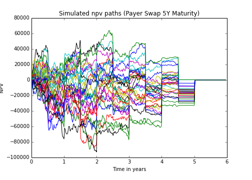
In the next step will we will floor each path at zero. This give the exposure of the portfolio on a path at each time. exposureSwap 
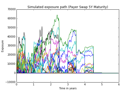
The expected exposure is given by the average of all paths: expExposureSwap 
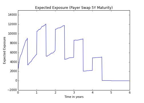
The total number of NPV evaluations is (size of time grid) x (size of portfolio) x N. For a big portfolio and a very dense time grid it can be very time consuming task even if the single pricing is done pretty fast.

Assumption made in this example

For simplicity we restrict the portfolio to plain vanilla interest rate swaps in one currency. Further we assume that we live in a “single curve” world. We will use the same yield curve for discounting and forwarding. No spreads between the different tenor curves neither CSA discounting are taken into account. For the swap pricing we will need future states of the yield curve. In our setup we assume the the development of the yield curve follow an one factor Hull-White model. At the moment we make no assumption on how it is calibrated and assume its already calibrated. In our setting we will simulate N paths of the short rate following the Hull-White dynamics. At each time on each path the yield curve depend only on the state of our short rate process. We will use QuantLib functionalities to simulate the market states and perform the swap pricing on each path. The calculation of the expected exposure will be done in Python.

Technical Implementation

1. Setup of the market state at time zero (today)

rate = ql.SimpleQuote(0.03)
rate_handle = ql.QuoteHandle(rate)
dc = ql.Actual365Fixed()
yts = ql.FlatForward(today, rate_handle, dc)
yts.enableExtrapolation()
hyts = ql.RelinkableYieldTermStructureHandle(yts)
t0_curve = ql.YieldTermStructureHandle(yts)
euribor6m = ql.Euribor6M(hyts)

As mentioned above we live in a single curve world, we use a flat yield curve as discount and forward curve. During the Monte Carlo Simulation we will relink the Handle to the yieldTermStrucutre htys to our simulated yield curve. The original curve is stored in yts and the handle t0_curve.

2. Setup portfolio / netting set

# Setup a dummy portfolio with two Swaps
def makeSwap(start, maturity, nominal, fixedRate, index, typ=ql.VanillaSwap.Payer):
    &quot;&quot;&quot;
    creates a plain vanilla swap with fixedLegTenor 1Y
    
    parameter:
        
        start (ql.Date) : Start Date
        
        maturity (ql.Period) : SwapTenor
        
        nominal (float) : Nominal
        
        fixedRate (float) : rate paid on fixed leg
        
        index (ql.IborIndex) : Index
        
    return: tuple(ql.Swap, list&lt;Dates&gt;) Swap and all fixing dates
    
        
    &quot;&quot;&quot;
    end = ql.TARGET().advance(start, maturity)
    fixedLegTenor = ql.Period(&quot;1y&quot;)
    fixedLegBDC = ql.ModifiedFollowing
    fixedLegDC = ql.Thirty360(ql.Thirty360.BondBasis)
    spread = 0.0
    fixedSchedule = ql.Schedule(start,
                                end, 
                                fixedLegTenor, 
                                index.fixingCalendar(), 
                                fixedLegBDC,
                                fixedLegBDC, 
                                ql.DateGeneration.Backward,
                                False)
    floatSchedule = ql.Schedule(start,
                                end,
                                index.tenor(),
                                index.fixingCalendar(),
                                index.businessDayConvention(),
                                index.businessDayConvention(),
                                ql.DateGeneration.Backward,
                                False)
    swap = ql.VanillaSwap(typ, 
                          nominal,
                          fixedSchedule,
                          fixedRate,
                          fixedLegDC,
                          floatSchedule,
                          index,
                          spread,
                          index.dayCounter())
    return swap, [index.fixingDate(x) for x in floatSchedule][:-1]

The method makeSwap create a new QuantLib plain vanilla swap (see my previous post). We use this method to setup a netting set with two swaps:

portfolio = [makeSwap(today + ql.Period(&quot;2d&quot;),
                      ql.Period(&quot;5Y&quot;),
                      1e6,
                      0.03,
                      euribor6m),
             makeSwap(today + ql.Period(&quot;2d&quot;),
                      ql.Period(&quot;4Y&quot;),
                      5e5,
                      0.03,
                      euribor6m,
                      ql.VanillaSwap.Receiver),
            ]

Our netting set consists of two swaps, one receiver and one payer swap. Both swaps differ also in notional and time to maturity. Finally we create a pricing engine and link each swap in our portfolio with it.

engine = ql.DiscountingSwapEngine(hyts)

for deal, fixingDates in portfolio:
 deal.setPricingEngine(engine)
 print(deal.NPV())

In our Monte Carlo Simulation we can relink the handle hyts and use the same pricing engine. So we don’t need to create new pricing engines or relink the the deals to a new engine. We just need to call the method NPV of the instruments after relinking the yield term structure handle.

3. Monte-Carlo-Simulation of the “market”

We select a weekly time grid, including all fixing days of the portfolio. To generate the future yield curves we are using the GSR model and process of the QuantLib.

volas = [ql.QuoteHandle(ql.SimpleQuote(0.0075)),
ql.QuoteHandle(ql.SimpleQuote(0.0075))]
meanRev = [ql.QuoteHandle(ql.SimpleQuote(0.02))]
model = ql.Gsr(t0_curve, [today+100], volas, meanRev, 16.)
process = model.stateProcess()

The GSR model allows the mean reversion and the volatility to be piecewise constant. In our case here both parameter are set constant. For a more detailed view on the GSR model have a look on the C++ examples “Gaussian1dModels” in the QuantLib or here. Given a time t_0 and state x(t_0) of the process we know the conditional transition density for x(t_1) for t_1 > t_0. Therefore we don’t need to discretize the process between the evaluation dates. As a random number generator we are using the Mersenne Twister.

#%%timeit
# Generate N paths
N = 1500
x = np.zeros((N, len(time_grid)))
y = np.zeros((N, len(time_grid)))
pillars = np.array([0.0, 0.5, 1, 2, 3, 4, 5, 6, 7, 8, 9, 10])
zero_bonds = np.zeros((N, len(time_grid), 12))
for j in range(12):
    zero_bonds[:, 0, j] = model.zerobond(pillars[j],
                                         0,
                                         0)
for n in range(0,N):
    dWs = generator.nextSequence().value()
    for i in range(1, len(time_grid)):
        t0 = time_grid[i-1]
        t1 = time_grid[i]
        x[n,i] = process.expectation(t0, 
                                     x[n,i-1], 
                                     dt[i-1]) + dWs[i-1] * process.stdDeviation(t0,
                                              x[n,i-1],
                                              dt[i-1])
        y[n,i] = (x[n,i] - process.expectation(0,0,t1)) / process.stdDeviation(0,0,t1)
        for j in range(12):
            zero_bonds[n, i, j] = model.zerobond(t1+pillars[j],
                                                 t1,
                                                 y[n, i])
                                                 

We also save the zero bonds prices on each scenario for a set of maturities (6M, 1Y,…,10Y). We use this prices as discount factors for our scenario yield curve.

4. Pricing on path & netting

On each date t and on each path p we will evaluate the netting set. First we build a new yield curve using the scenario discount factors from the step before.

date = date_grid[t]
ql.Settings.instance().setEvaluationDate(date)
ycDates = [date, 
           date + ql.Period(6, ql.Months)] 
ycDates += [date + ql.Period(i,ql.Years) for i in range(1,11)]
yc = ql.DiscountCurve(ycDates, 
                      zero_bonds[p, t, :], 
                      ql.Actual365Fixed())
yc.enableExtrapolation()
hyts.linkTo(yc)

After relinking the yield termstructure handle is the revaluation of the portfolio is straight forward. We just need to take fixing dates into account and store the fixings otherwise the pricing will fail.

for i in range(len(portfolio)):
    npv_cube[p, t, i] = portfolio[i][0].NPV()
5. Calculation EE and PFE

After populating the cube of fair values (1st dimension is simulation number, 2nd dimension is the time and 3rd dimension is the deal) we can calculate the expected exposure and the potential future exposure.

# Calculate the portfolio npv by netting all NPV
portfolio_npv = np.sum(npv_cube,axis=2)
# Calculate exposure
E = portfolio_npv.copy()
E[E&amp;amp;amp;lt;0]=0
EE = np.sum(E, axis=0)/N

Expected Expsoure Netting Set 
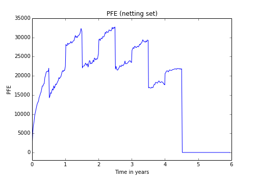
With PFE(t) we mean the 95 % quantile of the empirical distribution of the portfolio exposure at time t.

PFE_curve = np.apply_along_axis(lambda x: np.sort(x)[0.95*N],0, E)
MPFE = np.max(PFE_curve)

PFE netting set

Conclusion

With very few lines of code you can build a simulation engine for exposure profiles for a portfolio of plain vanilla swaps. These paths allows us to calculate the expected exposure or potential future exposure. Of course is the problem set in real world applications much more complex, we haven’t covered calibration (historical or market implied) or multi currencies / multi asset classes yet. And its getting even more complicated if you have multi-callable products in your portfolio.

But nevertheless I hope you have enjoyed reading this little tutorial and got an first insight into exposure simulation with QuantLib and Python. In one of my next post I will may extend this example about CVA calculation.

So long!