The post Effective Communication in Slack for Engineering teams appeared first on Leev's.
]]>I get it. Slack can be a distraction and, sometimes, a time waste. But this post will try to change some people’s minds around it. I’ll share some of the best tips and tricks I’ve found throughout my career. These practices transform Slack into a SUPERPOWER for Engineering teams, especially for those who provide internal services like Data or Platform teams.
To do that, let’s imagine you are the Engineering Manager for a Data Platform team consisting of several teams.
Channels Layout
Group Channels With Prefix
Slack channels can be organized based on categories (and if you are not doing it yet, please do), but the default ordering is alphabetical. This becomes handy if you apply the first trick – always use prefixes for your channels. In our case, we could use the acronym of Data Platform – dp as our channel prefix.
This will help our users find the right channel quickly, as all Data Platform channels will be marked with that prefix and in order on Slack. Within each group, teams share varying amounts of context. Quick navigation between channels becomes an easy win for your users.
Clear-Goal Channels
Keep your channels clean and tidy with the three-channel method. For every product we own, let’s say the Data Streaming Platform, we will have a support channel, update channel, and team private channel.
🔒dp-data-streaming-team
#dp-data-streaming-updates
#dp-data-streaming-support
🔒dp-data-analytics-team
#dp-data-analytics-updates
#dp-data-analytics-support
..
Support Channel
As the name suggests, this is your users’ go-to channel when they need to raise a request, ask for support, or raise an incident.
Later on in this post, we will cover this channel in more depth.
Update Channel
This read-only channel acts as your product change log. Find the right balance to avoid abusing this channel with non-actionable or critical messages. Your goal is to create “Pavlovian conditioning” for your users with this channel. Seeing a new message in that channel == I should check it out!
Going to apply a change to one of your Production clusters? Update the channel in advance, and keep it up-to-date in a thread. Need users to know of a new feature that will make their lives easier? Update in that channel.
Keep the messages concise and informative as much as possible. In your post-mortem, make sure you put a reference to that channel notification and you will immediately get 10 new joiners to that channel.
Private Channel
Just a friendly channel for our team to discuss day-to-day communication.
It might sound silly, but having this channel, even if your team consists of only two people, might become handy when a new joiner starts, or when someone decides to leave the team. Don’t underestimate the power of history. Context is the new gold. A quick search in Slack history might pop up some context worth discussion from the past, or a discussion on how to solve problem X.
Ace the Support Channel
As mentioned before, our support channel is one of the most crucial channels we have. We need to learn how to ace it in order to reduce the load on the teams in terms of support requests, task management, reduce context-switching, and give essential knowledge to your users.
Slack Workflows and Emojis
One of the best features in Slack, is Slack Workflows. This simple-yet-powerful tool allows you to create simple automation based on different sources and actions. One of them is millennials’ best friend – Emojis.
Try to think of all the repetitive responses and actions on the support channels, and automate them using emoji reactions. Questions like “how do I get permissions to do X?” could be answered with a “ ” emoji, which will add a bot comment in a thread pointing to the right document. Not enough context on a support request?, a “
 ” will trigger a comment to ask for more context, logs, and dashboard links. The possibilities are endless!
Project Management Integration
Spend some time integrating your company’s project management integration. Whether it’s Jira or Monday.com, all of them have integrations that will allow you to create tickets right from Slack.
This step will, once again, save some time on context-switching, plus, will give your users a way to track their issues, as most integrations will post the ticket link back to the channel.
Team Alignment and Mac Text Replacement
Using ad-hoc private chats for support is your worst enemy. It keeps the context within a pair of people and creates more load on a given person. It also prevents other team members from gaining insights from the answers. Those chats are like sticky sessions – the moment you answer one, the flood will follow and it becomes the go-to chat for a given user support.
This usually happens as people tend to be nice and helpful, but we need to make sure to clarify the importance of sending all requests to the support channel (like, sending this blog post to your team  ).
).
In our endless effort to save time and brain-compute-power on context switching, we can use the powerful Mac text replacement to point to our support channel. We can help our team members set it up to an agreed shared message. A quick text shortcut like "sprt" (support) plus Tab⇥ key will be replaced with a message like:
“Thanks for reaching out! In order to align our support process, can you please reach out to #dp-data-streaming-support? I’ll answer there!”
This simple and effective step will gradually prevent ad-hoc questions from reaching your teams and will log all the support requests into a single channel, where the most available person can help.
Bookmarks and Pinned Messages
Another useful feature of Slack is Bookmarks and Pinned Messages. This allows you to surface key links to your users – crucial documentation, Grafana dashboards, Jira boards, and more.
Someone asks “how to” questions but the answer lies in one of the bookmarks? Point them there, using Mac Text Replacement, of course.
What kind of documentation you should bookmark is outside the scope of this post, but I would highly recommend adding an “idiot-proof” debugging guide, representing the flow of your system and how to debug each component. By the end of that document, you can point users to the support channel with all the information gathered along the way. The guide provides users more exposure to the systems they’re using. Users gain independence to find and potentially fix their own problems. When system issues arise, you’ll receive much more context than “I have a problem with my data pipeline” as they could share the logs and findings.
Support Rota for New Team Members
Learn by helping others. Have your new team members handle incoming support requests in the channel. While they’ll need guidance, this hands-on approach is the best way to learn. It creates more learning opportunities than having senior team members quickly resolve support tickets.
Make it Data-Driven
Once you start implementing these steps in your organization, I can assure you that the impact will be visible. Your team members will be happier with the support routine, and the most magical moment of it all – your users will start answering each other.
A past colleague of mine implemented the method in his new role, and it resulted in success:

But let’s not stop here.
As data-driven professionals, we can get much more from our support channel.
Slack has a simple-to-use API, which allows you to export all the support requests and messages from the channel. By doing this, we get high-value insight into our users’ behavior and challenges.
Today, in the world of LLMs, everyone can become a data analyst within seconds. Start by analyzing the support channel – what are the hot topics? What are the challenges users are facing again and again?
Identifying these topics will give you the best insight of them all – a product which needs your attention again and again is either not good enough, too complex, or lacks proper documentation. Don’t neglect that.
To take it to the next step, we can automate that process to run and analyze once a month or a quarter. This can be especially helpful when planning the work for the next quarter, and the amount of BAU/KTLO (essential maintenance and operational routine work metrics) needed to be preserved by your team.
For the Data enthusiasts out there, a cool way to represent these keywords is in a word cloud graph!

You can easily transform those insights into a team KPI, with a clear goal of lowering the amount of requests on a given topic.
Conclusion
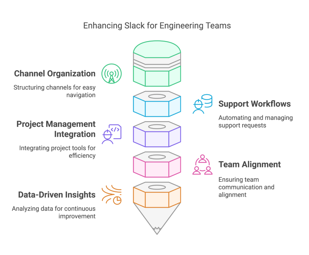
In this post, we explored how to transform Slack from a potential distraction into a powerful tool for engineering teams. By implementing structured channel layouts, automating support workflows, and leveraging data-driven insights, teams can significantly improve their communication and efficiency.
Remember, the key is not just using Slack, but using it strategically to enhance team collaboration and productivity.
And for the Actionable plan:
| Time Frame | Action | Description |
|---|---|---|
| Week 1 | Channel Organization | * Create standard channel prefixes for your team/product * Set up support, updates, and private channels * Share the structure with your team |
| Week 2-3 | Support Workflows | * Configure emoji-based workflows for common requests * Set up project management integration * Share response templates and Mac shortcuts |
| Week 3-4 | Documentation | * Pin debugging guides and crucial documentation * Set up channel bookmarks * Establish update channel guidelines |
| Month 2 | Analytics, and repet | * Set up Slack API for support channel data collection * Create monthly review process * Track KPIs: response times, resolution rates |
The post Effective Communication in Slack for Engineering teams appeared first on Leev's.
]]>The post How to debug Strimzi Kafka Connect Connector appeared first on Leev's.
]]> Quick Tip Post
 Usually, this blog contains long, deep-dive posts. This category will be different! This is a short and actionable post, which otherwise would go to /dev/null
Strimzi is awesome! In the last few years, it has made huge progress, becoming the go-to option to run the Kafka ecosystem on top of Kubernetes.
But as with every other JVM-based system, from time to time, we just need to use our old favourite tools like JConsole and Java Flight Recorder. When it comes to Kubernetes, it’s a bit more tricky.
In order to connect to a running Kafka Connect pods (running a Kafka Connect Connector or Debezium) with tools like JConsole, JMX Term, or Java FlightRecorder, we will need to expose the JMX ports locally and run a Kubernetes port-forward.
To do that, we will expose the JMX port, and override some of the parameters:
image: strimzi/kafka-connect:0.11.4-kafka-2.1.0
jmxOptions: {}
jvmOptions:
…
template:
   connectContainer:
      env:
      - name: KAFKA_OPTS
      value: -Dcom.sun.management.jmxremote.local.only=false -Djava.rmi.server.hostname=127.0.0.1
The important ones are jmxOptions and KAFKA_OPTS.
- We use
jmxOptions: {}to make sure we expose the JMX port without any auth. - The
KAFKA_OPTSparameter allows us to add some flags to the JVM. In this case, allowing connections from “outside”, and exposing it to localhost. The base config for JMX is configured on Strimzi startup scripts, which does not allow us to configure them to allow outside connections, thus, we need to make these changes as well.
Once we have it, you can use the tools to connect to the running pods using a simple kubectl port-forward:
Start JConsole
kubectl port-forward <strimzi_pod> 9999
jconsole -J-DsocksProxyHost=localhost -J-DsocksProxyPort=9999 service:jmx:rmi:///jndi/rmi://localhost:9999/jmxrmi
Start JMXTerm
If you are not familiar with JMXterm, go over Robin Moffatt‘s great post:
java -jar jmxterm-1.0.2-uber.jar --url localhost:9999Java Flight Recorder
JFR is a bit more tricky.
Once again, we need to edit our KafkaConnect object with:
jvmOptions:
  -XX:+UnlockDiagnosticVMOptions
  -XX:+DebugNonSafepoints
  -XX:+UnlockCommercialFeatures
  -XX:+FlightRecorder
  -XX:StartFlightRecording=filename=/tmp/recording.jfr,duration=60s
...
...
template:
  connectContainer:
    env:
      - name: KAFKA_OPTS
        value: "-Dcom.sun.management.jmxremote.local.only=false -Djava.rmi.server.hostname=127.0.0.1"
To start and stop the JFR sessions:
# start
kubectl exec -it <strimzi_pods> -- jcmd <pid> JFR.start name=myRecording filename=/tmp/recording.jfr duration=60s

# list
kubectl exec -it <strimzi_pods> -- jcmd <pid> JFR.check

# stop
kubectl exec -it <strimzi_pods> -- jcmd <pid> JFR.stop name=myRecording
Once we have the recording ready, we can use cp to retrieve it and analyse it locally:
kubectl cp <strimzi_pods>:/tmp/recording.jfr ./recording.jfr
jmc
From JMC, load the recording.jfr file and analyse the performance metrics.
Done! Happy debugging! 
The post How to debug Strimzi Kafka Connect Connector appeared first on Leev's.
]]>The post Bridging the gap between eras using Debezium and CDC appeared first on Leev's.
]]>But not all systems were born equal, and when dealing with legacy systems – achieve that could be quite a challenge, and might involve some scalability issues? How can you transform it into a reactive component?
Let’s start with the basics –
Batch vs Streaming
There’s a well-known saying about distributed systems: because of the complexity they bring, you should only use them when absolutely necessary. In a way, the same goes for Data Streaming which is more complex compared to batch processing. In a batch system, we process known finite-size inputs. We can always fix a bug in our code, and replay the batch. But in a stream, we process unbounded datasets which have no beginning and end.
Having said that, from a business perspective, there are clear benefits from using streaming instead of batching as in many cases, a business event loses its value over time.

A good example of this is fraud detection services – Detecting fraudulent activities, such as credit card fraud or cybersecurity threats, requires immediate action to prevent further damage. Batch processing of transaction data introduces delays, during which fraudsters can continue their malicious activities. Streaming analytics enable real-time fraud detection systems to identify suspicious patterns as they occur, allowing for instant alerts and preventative measures.
The closer we can bring the action-taking to the business event, the better.
But what can you do if a legacy system is involved as part of the pipeline? A system that doesn’t “know” how to stream. In our case, an old ETL pipeline which is sourced from a legacy Oracle database.
Introducing, Change Data Capture
One of the ways to overcome this problem is by leveraging a common data pattern called “Change Data Capture” (CDC). It allows us to transform any static database into an event stream we can act upon.
The CDC process includes listening, identifying and tracking changes occurring in a database, and creating an event based on them.
CDC can be implemented using three main methods – Trigger based, Query based and Log based CDC.
A trigger-based CDC works by employing database triggers. In this approach, triggers are set up on tables within a database, and they are designed to activate automatically in response to specific data manipulation events, such as INSERT, UPDATE, or DELETE operations.
Query-based CDC, works by periodically querying the source database for any modifications. It is mainly used when direct modification of the source database is not feasible.
The last, and most efficient one is the log-based CDC. This approach leverages database transaction logs to capture and track changes made to data in a source database. This approach provides a near-real-time and efficient way to identify modifications, additions, or deletions without putting a significant load on the source database.
Debezium
When dealing with CDC and databases, the most common tool for the job is Debezium.
“Debezium is a set of distributed services that capture row-level changes in your databases so that your applications can see and respond to those changes. Debezium records in a transaction log all row-level changes committed to each database table. Each application simply reads the transaction logs they’re interested in, and they see all of the events in the same order in which they occurred.”
Debezium documentation
Debezium is actively maintained and supports the most common databases in the world – MySQL, MongoDB, PostgreSQL, Oracle, Spanner, and more.
Although you can run Debezium as a standalone Debezium Server or inside your JVM-based code using Debezium Engine, the most common practice is to deploy it as a Connector on top of a Kafka Connect cluster to leverage the benefits of the platform like orchestration, parallelism, failure handling, monitoring, and more.

Problem Statement
Our story begins with an old ETL pipeline which gets a dump of data every day, and later on loaded and processed on our data platform.

On the left side, we have the source backend which contains the Oracle database. Once a day, a new dump of the data is transferred to the landing bucket for processing.
On the right side, we have a service which holds the “Processing Logic”, that is, loading the data from the landing bucket, doing some data transformation and cleanup, making some business operations, and finally ingesting the result dataset to the Data Warehouse.
As data consumers, we have some ML Models, Data Analysts, and operational dashboards.
To begin with, we need to identify the problems with this solution:
As mentioned before, there are some obvious downsides to using such a method. As we deal with a daily batch of data, the freshness of our data is low.
Then, there are scalability issues and error handling. As companies continue to grows, the data volumes keep piling up to a point where the batches we process might take way too long to complete. It affects both the operation and business side – recovering from an error and re-processing a batch takes much longer over time, and our business decision-making is slower.
Now let’s make it better with Debezium!
The new architecture is fully based on Kafka, Kafka Connect and Debezium, to power (near) real-time ingestion to the Data Warehouse:

Instead of getting a daily dump of the data and processing it with an in-house service, we can leverage open source technologies which are developed and tested by thousands of engineers around the world.
In the new solution, the Debezium Oracle Connector is hosted on the Kafka Connect platform which simplifies the orchestration, scaling, error handling, and monitoring of such services. The connector is using Oracle LogMiner to query the archived and offline redo logs to capture the history of activity in the Oracle database.
Using Kafka Connect SMTs (more on that later), we can clean up and transform our CDC messages, and ingest them into Kafka.
To ingest the data into BigQuery and GCS, we can simply use another open-source Kafka connectors, which we can now scale independently.
The new pipeline is far more efficient, allows us to capture changes in real time, and reduces most of the complexity of the old pipeline. No service to maintain, battle-tested connectors and platform, a simple way to transform data, and the ability to independently scale each one of the components in the system.
Debezium Snapshot
On Oracle, the redo logs usually do not retain the full history of the database from the dawn of history. Consequently, the Debezium Oracle connector cannot access the entire database history from these logs. To allow the connector to create a baseline of the current database state, it takes an initial consistent snapshot of the database when it starts for the first time. This process can be controlled via a parameter called [snapshot.mode].
During the startup procedure, Debezium obtains a ROW SHARE MODE lock on each of the captured tables to prevent structural changes from occurring during the creation of the snapshot. Debezium holds the lock for only a short time.
Data Change Events
Once Debezium starts to capture all changed data (CREATE, UPDATE, DELETE, TRUNCATE), we will get the data change events to Kafka. Every data change event that the Oracle connector emits has a key and a value.
An expected CREATE event might look like the following:
{
    "schema": {
        "type": "struct",
        "fields": [....],
        "optional": false,
        "name": "server1.DEBEZIUM.CUSTOMERS.Envelope"
    },
    "payload": {
        "before": null,
        "after": {
            "ID": 1004,
            "FIRST_NAME": "Anne",
            "LAST_NAME": "Kretchmar",
            "EMAIL": "[email protected]"
        },
        "source": {
            "version": "2.6.1.Final",
            "name": "server1",
            "ts_ms": 1520085154000,
            "ts_us": 1520085154000000,
            "ts_ns": 1520085154000000000,
            "txId": "6.28.807",
            "scn": "2122185",
            "commit_scn": "2122185",
            "rs_id": "001234.00012345.0124",
            "ssn": 1,
            "redo_thread": 1,
            "user_name": "user",
            "snapshot": false
        },
        "op": "c",
        "ts_ms": 1532592105975,
        "ts_us": 1532592105975741,
        "ts_ns": 1532592105975741582
    }
}
In same cases, this is exactly what you would need – a stream of changes that an external system can consume. In this case, I don’t really need the extra information, and I simply want to replicate those events into Kafka while doing some basic transformations.
To do that, we can leverage Single Message Transformations.
Single Message Transformations
Single Message Transformations (SMTs) are applied to messages as they pass through Kafka Connect. SMTs modify incoming messages after a source connector generates them but before they are written to Kafka. They also transform outgoing messages before they are sent to a sink connector.
You can find more about SMTs in Debezium or Confluent documentation, but SMTs can be as easy as:
"transforms": "ExtractField",
"transforms.ExtractField.type": "org.apache.kafka.connect.transforms.ExtractField$Value",
"transforms.ExtractField.field": "id"
The configuration snippet above shows how to use ExtractField to extract the field name "id"
Before: {"id": 42, "cost": 4000}
After: 42
In this case, we want to strip out most of the excess metadata, and only keep the value of the “after” event – as, the updated value, and some extra fields like ts_ms and scn for tracking.
To do so, we simply use the unwrap SMT:
    transforms: unwrap
    transforms.unwrap.type: io.debezium.transforms.ExtractNewRecordState
    transforms.unwrap.add.fields: source.ts_ms,ts_ms,scn
Now each one of our events in Kafka will consist of a key and a clean value.
Extend with a Custom SMT
Assuming one of our down-stream systems needs to make an aggregation based on the key of the messages, but it has only access to the message value. Can we fix it with SMT? Yes!
Unfortunately, there is no SMT which can take the message key and insert it as a field in the value, but SMTs are built the same way as the whole Kafka Connect platform – predefined interfaces which are easy to extend.
Introducing – KeyToField – SMT for Kafka Connect / Debezium.
With this custom SMT that I built, we can do exactly that – add the message key as a field. The SMT can also handle complex keys with multiple fields in it, using the transforms.keyToField.field.delimiter variable that will be used when concatenating the key fields.
A custom SMT can be as easy as a single Java file implementing the relevant methods.
@Override
    public R apply(R record) {
        if (record.valueSchema() == null) {
            return applySchemaless(record);
        } else {
            return applyWithSchema(record);
        }
    }
The apply method gets the record and perform the action based on the record schema (or schema-less).
We update the schema, put the new field as a string, and return the new record with the new schema and value:
private R applyWithSchema(R record) {
        ...
        updatedSchema = makeUpdatedSchema(value.schema());
        ...
        final String keyAsString = extractKeyAsString(record.keySchema(), record.key());
        updatedValue.put(fieldName, keyAsString);
        return record.newRecord(
                record.topic(),
                record.kafkaPartition(),
                record.keySchema(),
                record.key(),
                updatedSchema,
                updatedValue,
                record.timestamp()
        );
    }
as simple as that.
Our final SMT configuration now looks like:
transforms: unwrap,insertKeyField
# Extract record
transforms.unwrap.type: io.debezium.transforms.ExtractNewRecordState
transforms.unwrap.add.fields: source.ts_ms,ts_ms,scn
# Add key as field
transforms.insertKeyField.type: com.github.eladleev.kafka.connect.transform.keytofield.KeyToFieldTransform
transforms.insertKeyField.field.name: PK
With that, our pipeline is complete and relatively straightforward – Debezium generates the events from the source database, we transform the data using SMTs, ingest them to Kafka, and from there we have two connectors taking care of the ingestion to Big Query and GCS.
Conclusion
Dealing with legacy systems that rely on batch processing introducing a significant challenges in terms of data freshness, scalability, and timely business decision-making.
The transition to a modern data architecture leveraging Change Data Capture (CDC) with Debezium and Kafka addresses these issues effectively. By capturing and streaming real-time changes from the legacy Oracle database to Kafka, we significantly enhance data freshness and reduce latency. This new architecture facilitates near-real-time data processing and decision-making, enabling businesses to respond quicker.
In summary, the integration of Debezium and CDC into the data pipeline transforms a legacy batch processing system into a reactive, real-time data streaming architecture. This shift not only improves data freshness and scalability but also enhances the overall efficiency and responsiveness of the business, paving the way for more informed and timely decision-making.
The post Bridging the gap between eras using Debezium and CDC appeared first on Leev's.
]]>But I feel that there is a profound problem with Terraform that no one talks about, or states enough.
The post The profound problem with Terraform we are not talking about appeared first on Leev's.
]]>It’s been a while, but I’ve been there from the happy days of Bash and Perl scripts to the rise (and fall) of Puppet ( )/Chef/Ansible, the Terraform revolution, and the new era of control planes, operators and Kubernetes.

With almost 2 billion downloads over time to the official AWS provider, it’s safe to say that Terraform is de facto the gold standard for IaC. It also plays a key role as the bridge between eras – companies who still use traditional CM systems mix it with Terraform, and companies that are fully invested in Cloud Native and K8s, still use Terraform, because of the natural difference between the two.
Terraform is awesome. It really is. Although many people complain about HCL, the non-trivial state management, and the toil involved in using the tool, it gets the job done and does it well. It has a much shorter learning curve than K8s and with the right modules, you can easily create a dead-simple facade for your infrastructure that even non-developers can deal with in a few minutes.
But I feel that there is a profound problem with Terraform that no one talks about, or states enough.
Something is fundamentally broken with the process of plan and apply.
It’s not always the case, but based on my experience, I find it way too common – you create your Terraform project, use community or self-developed modules, run plan, create a PR, get an approval, and everything looks promising – you double and triple check your plan output, and you hit the merge button.
Surprise surprise — Terraform failed.
How could it be? Despite checking my code many times, asking my peers for a review, we all saw the plan output, but it did not help – still a failure.
This strange and annoying discrepancy is not necessarily Terraform’s problem, but we have all faced it before. The main reason is the fact that most of the time, the only moment Terraform is actually making an action is during the apply stage.
When you apply a resource, you might face unexpected results from the underlined APIs. During the plan phase, Terraform performs only basic static checks against your code, but once you apply, you are facing some vendor-related nuances. Suddenly, the labels you set do not match the supported Regex. It’s not kebab-case/snake_case/camelCase (thank you for your inconsistencies, GCP). The resource name is longer than 28 character, or any other problem that might pop out only during the call to the actual API.
It’s not just frustrating. It’s also breaking the basic rule of modern GitOps – our main branch is not representing reality anymore. It’s no longer the source of truth, as we just merged unapplied changes.
It’s not all terrible, there is a solution to the problem. Some APIs and providers implement some kind of dry-run as part of their planning process, or variable validations based on pre-known restrictions and limitations.
But, if that’s not the case with some of the world’s leading cloud providers like AWS and GCP, how can we expect that from much smaller vendors or community modules?
Vendors need to understand that this is the entry point to their services and treat it like they should. The same as we won’t promote un-tested or low-test-coverage code to production, the same holds true for official modules – put in the extra effort. Cover the edge cases. Add validations. Support dry-running on your API. Do dogfooding. Invest in proper documentation.
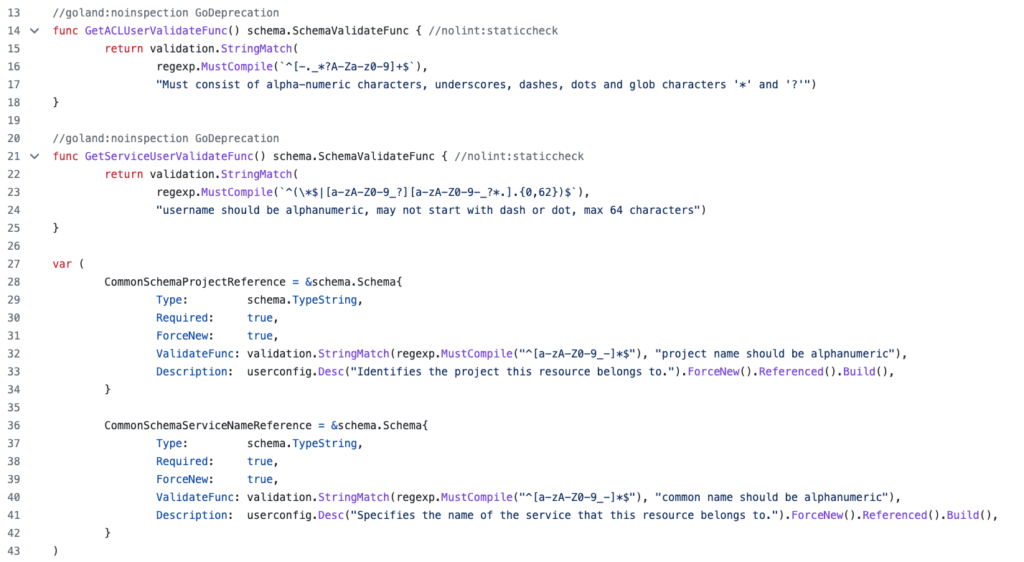
ValidateFunc by Aiven provider.We can’t really expect action from Hasicorp itself, as Terraform attempts to take into account as much known information as possible during the plan phase, and there are no magic bullets.
What we can expect, demand and contribute for, is more robust and bulletproof plugins and providers, that will prevent this situation.
In conclusion, while Terraform is a fantastic tool, the plan and apply process can be frustrating due to unexpected API results. To address this issue, cloud providers and module developers should invest in proper documentation, edge case coverage, and validation rules. This will prevent surprises during the apply phase.
It is up to us as users to demand and contribute to more robust and bulletproof plugins and providers.
Sorry for the clickbait in the title .
The post The profound problem with Terraform we are not talking about appeared first on Leev's.
]]>The post Know Your Limits: Cluster Benchmarks appeared first on Leev's.
]]>This post originally appeared on Riskified Technology Blog
“No single metric can measure the performance of computer systems on all applications. System performance varies enormously from one application domain to another. Each system is typically designed for a few problem domains and may be incapable of performing other tasks.”
Jim Gray, “The Benchmark Handbook for Database and Transaction Systems”, 1991.
Measuring system performance is hard – there are no magic bullets.
A design decision that you’ve made naively, like choosing the wrong instance type, may lead to degraded performance and even unavailability of your services later on as you scale. Something that’s not acceptable in today’s online world.
In his book from 1991, Jim Gray defines “how to choose the right system” perfectly – “The system that does the job with the lowest cost-of-ownership”.
Many companies only evaluate TCO (Total Cost of Ownership) when testing new products. They rely on their vendor benchmarks, which might be misleading (like network packets that are faster than the speed of light), or too broad (like AWS “up-to” magic phrase when dealing with network performance).
Despite the fact that there are many useful analysis reports, which are more focused on pushing distributed systems to their limits, like the famously known Jepsen, it is important to know your own custom deployment limiting factor as it might be different from one deployment to another.
Knowing how much your system can handle, how many RPS it can make and what the limiting factor is – the disk, network, memory or CPU can give your deployment a better framing, assist in preventive maintenance and help you guesstimate the impact of scaling out your system and eliminating toil.
Riskified’s Data Platform
Riskified’s Data Platform group is split into 3 teams – Data Offline, Data Apps, and the bridge between them – Data Streams. Each team is responsible for its own specific data domain.
Our main goal is to provide an efficient, robust and scalable data platform that is used by hundreds of Riskified employees in the various departments – Development, Data Engineering, BI, Data-Science, Research, Support & Integrations, and more.
As we continue to grow, the amount of data we process, store and analyze grows too, and the demand on our systems only gets higher as a result.
We aim to provide the highest SLA possible to our internal clients, allowing them to move fast and only focus on the thing that matters – the business logic itself.
With that in mind, and with plans to migrate into a new Kafka deployment that will allow us to move faster, we decided to apply the same method, and benchmark our clusters before migrating into them.
Setting the goals
We started to plan our cluster benchmark with a few key points in mind:
- No special tricks – the benchmark should test the exact same deployment and configuration as we planned to use on our new clusters
- Mimic our environment – the benchmark should run as a Riskified service from our K8S cluster, with the same resources that a real service would get
- It must measure the peak performance of the system when performing typical operations – in our case, producing and consuming from Kafka using the most commonly used client configurations
- Scalable – we need to have the ability to scale out and in the benchmark, to parallel tasks and to test different workloads on the same system as it evolves (i.e, adding more nodes and seeing the impact)
- Simple – the benchmark must be understandable, otherwise it will lack credibility
We defined a few key factors that are configurable by our clients and might affect the overall performance, and started to research what their most widely used values are.
We took into consideration our largest services (as our main internal clients) alongside the common values. Using that information, we created some kind of “Cartesian Product” with the different configuration combinations that we want to test against our cluster.
From our perspective, our baseline remains the performance of n-2, as we want to tolerate node failures and still be fully operational and keep the SLOs we defined as a team.
Having said that, we did test the final number of nodes that are going to be part of the new clusters.
We see this overhead-keeping as a best practice in our capacity planning.
What are the options?
After defining the goals and the tests suites, we started to evaluate the different options available for the task.
kafka-*-perf-test scripts
The most obvious first option was the built-in Kafka performance test tool. The tool allows you to measure, read and write throughput, stress test the cluster based on specific parameters, and more.
Apache JMeter
Apache JMeter is a veteran Apache project that can be used as a load testing tool for analyzing and measuring the performance of a variety of services.
Sangrenel
Sangrenel is a Kafka cluster load testing tool created by Jamie Alquiza (from DataDog). Sangrenel allows you to set the message and batch size, concurrency and other settings, and measure the message throughput, batch and write latency histograms.
OpenMessaging Benchmarks (OMB)
The OMB Framework is a suite of tools that make it easy to benchmark distributed messaging systems in the cloud.
Of all the available options, we decided to use the OpenMessaging Benchmarks tool.
The tool itself fulfills all the requirements and goals that we mentioned earlier, will be scalable enough and also will allow us to test other streaming platforms in the future, like Pulsar or NATS.
Define & build
As mentioned above, we wanted the benchmark to run as close to a real Riskified service as possible. That’s why we started by customizing the Helm chart, provided with the tool, to fit our environment and needs.
The OMB Framework is composed of two components – the driver and the workers.
The driver is responsible for assigning the tasks to the workers, creating the benchmark topic, creating the consumers and the producers, etc. Essentially it is the benchmark executor.
A benchmark worker listens to tasks to perform them. A worker ensemble communicates over HTTP.

In our deployment, we created a single pod that acts as the Driver and a StatefulSet of workers with the amount of replicas that we want to test depending on the parallelism.
The driver is executed by getting 2 manifests:
- The drive configurations – contain all consumer and producer configurations (
acks,linger.ms, compression type, etc.) - The workload configuration – sets workload characteristics. including topic name, message size, partitions per topic, producer rate, and more
After the execution, the driver starts to produce warm-up traffic, and then the benchmarking traffic itself, while logging the current results – publishing rates, consuming rates, backlog, and end-to-end latencies. At the end of the execution stage, aggregated metrics will appear.
The aggregated test results can be stored as a CSV file for later data analysis, and the tool is packed with a Python script to visualize the test results in a graph.
Benchmark Insights
As we ran the different workloads, we were able to discover our deployment average latency. We noticed how more partitions or more workers affect the benchmark latency and the cluster load.
Other than the output of the tool itself, we also tracked the cluster behavior using our Grafana dashboards. Using those, we were able to see how our dashboard behaved in extreme circumstances.
We were able to discover our potential bottlenecks, in our case, the EBS drives who suffered from the high flush rate that the benchmark created, and reflected it with high IO times, and as a consequence – a spike in the end to end latencies.
With those results, we are now much more confident in our deployments. We know what could possibly go wrong, what our limiting factor is, and on what stage (RPS, MB/s, etc).
Given that information, we made sure that we have actionable alerts when getting closer to that limit. We now know how adding more machines can affect the cluster, and how we can plan accordingly for high traffic seasons.
We discovered that our deployment with our existing traffic only covers a small part of our cluster potential in terms of resources. We believe that with the current growth rate, the current deployment could take us a few more months before the need to scale.
Future work
The fact that we battle-tested our cluster not only gave us more confidence, it also affected our roadmap and allowed us to better plan our future deployments.
For instance, we now have concrete numbers on how switching to Zstandard compression can lead to lower resource utilization, and will allow us to “squeeze” more information on to the network bandwidth.
We now know that we will need to reevaluate our usage of EBS drives at some point – everything is a tradeoff.
Setting clear goals, choosing the right tool and investing in research and tests, lead us to insightful information and will allow us to use the same techniques in the future, as part of our routine and with other systems that we will want to evaluate.
The post Know Your Limits: Cluster Benchmarks appeared first on Leev's.
]]>The post A Practical Guide for Kafka Cost Reduction appeared first on Leev's.
]]>Kafka is no different in that matter. Organizations all over the world are using Kafka as their main stream-processing platform for collecting, processing, and analyzing data at scale. As organizations evolve and grow, data rates grow too, as does the consequent cloud cost.
So what can we do? Is there any low-hanging fruits we can implement in order to cut some costs?
Here are few tips and KIPs (Kafka improvement proposals) that might help!
Disclaimer
This post is not going to cover the managed services method of cutting costs.
In some use cases, managed services like Confluent Cloud might do the trick.
For more information on that, you can refer to Cost Effective page on Confluent website.
Before we get started, we need to understand some basics.
What are we paying for?
I can try to list all the components that we are paying for when using the various cloud providers out there, but I won’t be able to do it as well as Gwen Shapira in her post “The Cost of Apache Kafka: An Engineer’s Guide to Pricing Out DIY Operations” –
Start with some fairly obvious and easy-to-quantify expenses
If you are going to run Kafka on AWS, you’ll need to pay for EC2 machines to run your brokers. If you are using a Kubernetes service like EKS, you pay for nodes and for the service itself (Kubernetes masters). Most relevant EC2 types are EBS store only and Kubernetes only supports EBS as a first-class disk option, which means you need to pay for EBS root volume in addition to the EBS data volume. Don’t forget that until KIP-500 is merged, Kafka is not just brokers — we need to run Apache ZooKeeper too, adding three or five nodes and their storage to the calculation. The way we run Kafka is behind a load balancer (acting partially as a NAT layer), and since each broker needs to be addressed individually, you’ll need to pay for the “bootstrap” route and a route for each broker.

All these are fixed costs that you pay without sending a single byte to Kafka.

On top of this, there are network costs. Getting data into EC2 costs money, and depending on your network setup (VPC, private link, or public internet), you may need to pay both when sending and receiving data. If you replicate data between zones or regions, make sure you account for those costs too. And if you are routing traffic through ELBs, you will pay extra for this traffic. Don’t forget to account for both ingress and egress, and keep in mind that with Kafka, you typically read 3–5 times as much as you write.

Now we are running the software, ingesting data, storing it, and reading it. We’re almost done. You need to monitor Kafka, right? Make sure you account for monitoring (Kafka has many important metrics)—either with a service or self-hosted, and you’ll need a way to collect logs and search them as well. These can end up being the most expensive parts of the system, especially if you have many partitions, which increases the number of metrics significantly.
I highlighted the main points from the post, and there are other components from the Kafka eco-system that are not directly mentioned, like Schema Registry, Connect workers, as well as tools like CMAK or Cruise-Control, but it will be applicable to the same three factors-
Machines, Storage, and Network.
While there are more factors that are much harder to measure, like employee salaries, down-times, and even dealing with interrupts (aka – the work that must be done to maintain the system in a functional state), those are the main factors that we pay for when using a cloud provider.
What can we do?
Beside some basic concepts that are applicable to almost every distributed system, over time, Kafka’s committers introduced a few KIPs and features that directly or indirectly affect Kafka’s TCO.
But we will still start with the obvious ones –
Are you using the right instance types?
There are plenty of instance types to choose from on AWS (you can use the same ideas on other cloud providers of course).
Kafka can run easily and without any apparent problems on inexpensive commodity hardware, and if you will Google the recommended instance types for a production-grade Kafka cluster, you would find r4, d2 or even c5 combined with GP2/3 or IO2 storage as the broad recommendation.
Each one has its own pros and cons, and you probably need to find the right one for you based on various tradeoffs—a longer time-to-recover (HDD disks), storage-to-dollar ratio, network throughput, and even EBS performance degradations in extreme circumstances.
But over time, i3 and i3en machines were added to that list, and based on my experience, they are by far the most recommended instance types based on ROI for large-scale deployments, even if you are taking into consideration the operational overhead of using ephemeral drives.
i3 and i3en provide better performance on an endless amount of benchmarks when using Kafka, and leverage the ephemeral drive advantages (10gbps disk bandwidth vs 875mbps on EBS-optimized C-class instances).
This great post by ScyllaDB examines how using i3en machines are much cheaper on systems where the main limiting factor is storage capacity (more on that later) –

As the first step of cost reduction, you will need to re-evaluate your instance type decision: Is your cluster saturated? In what condition? Are there other instance types that might fit better than the one you chose when you first created the cluster? Does the mixture of EBS-optimized instances with GP2/3 or IO2 drives really cost less than i3 or i3en machines and their advantages?
If you are not familiar with this tool, you should be.
Update for 2022: Today, the maturity of Graviton2 instances has proven itself. You might consider using these instance families as well! – It’s already running successfully in production in dozen of companies. You can start here.
As for non-graviton instances, AWS announced the new i4i instance family, which has already been tested by ScyllaDB and looks very promising (although, I’ll always recommend waiting a bit longer before migrating production clusters to new instance families).
Compression
Compression is not new in Kafka, and most of the users already know that you can choose between GZIP, Snappy and LZ4. But since KIP-110 was merged and added codec for Zstandard compression, it enabled a significant performance improvement, and a perfect way of reducing costs on networking.
Zstandard is a compression algorithm by Facebook; it aims for a smaller and faster data compression when compered to other compression algorithms.

For example, using zstd (Zstandard), Shopify was able to get 4.28x compression ratio. Another great example on the impact that zstd can make is “Squeezing the firehose: getting the most from Kafka compression” from Cloudflare.
And how is that relate to cost reduction? At cost of slightly higher CPU usage on the producer side, you will get a much higher compression ratio and “squeeze” more information on the line.
Amplitude describes in their post that after switching to Zstandard, their bandwidth usage decreased threefold, saving them tens of thousands of dollars per month in data transfer costs just from the processing pipeline alone.
You are paying for data transfer costs as well, remember?
Fetch from closest replica
It is common to spin your clusters on few availability zones within the same AWS region for fault tolerance.
Unfortunately, it is impossible to coordinate the placement of the consumers to be perfectly aligned with the leader of the partition that they need to consume in order to avoid cross-zone traffic and costs. Enters KIP-392.
Enabling rack awareness is possible since KIP-36 back in 2015, and can be easily done by adding a single line to your configuration file:
broker.rack=<rack ID as string> # For example, AWS AZ IDBefore KIP-392 was implemented, this setting controlled only the replica placement (by treating the AZs as a rack). However, this KIP addresses exactly this gap, and allows you to leverage locality in order to reduce expensive cross-dc traffic.
Some clients have already implemented the change, and if your client is not yet supporting it, here’s an open source project for your weekend! 
Cluster Balance
It might seem not that obvious, but your cluster imbalance might impact the cost of your cluster as well.
An imbalanced cluster might hurt the cluster performance, lead to brokers who are working harder than others, make response latency higher, and in certain circumstances lead to resource saturation on those brokers, and unnecessary capacity addition as a result.
Another risk you are exposed to with imbalanced clusters is higher MTTR after a broker failure (e.g., if that broker holds more partitions unnecessarily), and an even higher risk of data loss (imagine topics with a replication factor of 2, where one of the nodes struggle to start due to the high number of segments to load on startup).
Don’t let this relatively easy-to-do task become a money waste. You can use tools like CMAK, Kafka-Kit, or better yet, Cruise-Control, which allows you to automate these tasks based on multi goals (capacity violation, replica count violation, traffic distribution, etc.).
Fine tune your configuration – producer, brokers, consumers
Sounds obvious, huh?
But under the hood of your friendly Kafka clusters, there are tons of settings you can enable or change.
These settings can dramatically affect the way your cluster works: resource utilization, cluster availability, guarantee, latency, and many more.
For example, misbehave clients can impact your brokers resource utilization (CPU, disk, etc). Changing your clients batch.size and linger.ms (where business logic fits) can drop your cluster LoadAvg and CPU usage dramatically.
Message conversions introduce a processing overhead, since messages between the Kafka clients and brokers require conversion in order to be understood by both parties, leading to higher CPU usage. Upgrading your producers and consumers can solve this issue and free resources that were used unnecessarily for this task.
The number of examples are endless.
With the right fine tune, you can make your cluster work better, serve more, increase throughput, free up resources, and as a result avoid unnecessary capacity addition or even scale down your cluster to the right size for your needs.
It would be an impossible mission to read and process every line of the documentation, so you can start by reading one of the posts about tuning your clients and brokers. I would recommend the Strimzi series about it – Brokers, Producers, and Consumers.
The Future
Compression levels
As mention earlier, using one of the compression algorithms (preferably zstd) can give you great performance improvement and save you money on data transfer.
Dealing with compression introduce you to a new kind of trade-off that you need to decide on – CPU vs IO (the result compressed size). Most of the algorithms provide some kind of compressions level to choose from, which affects the amount of processing power required, and the result compresses dataset.

Until now, Kafka supported only the default compression level per codec. This aim is to be resolved on KIP-390 which will be shipped with Kafka 3.0.0.
After the KIP is implemented we will be able to add a single line to our configuration, and set the compression’s level higher (where it fits. Remember the resource overhead)
compression.type=gzip
compression.level=4             # NEW: Compression level to be used.
The new feature tested against a real-world dataset (29218 JSON files with an average size of 55.25kb), and the result may vary based on the various coded, compression levels, and the resultant latency as you can see below

Tiered Storage
The total storage required on a cluster is proportional to the number of topics and partitions, the rate of messages, and most importantly the retention period. Each Kafka broker on a cluster typically has a large number of disks results in 10s of TBs on a single cluster. Kafka has become the main entry point of all of the data in organizations, allowing clients not only consume the recent events, but also older data based on the topic retention.
It’s likely that more brokers or disks will be added, just to be able to hold more data on your clusters based on your client’s needs.
Another common pattern is to split your data pipeline into smaller clusters, and set a higher retention period on the upstream cluster for data recovery in case of a failure. Using this method, you will be able to “stop” the pipeline completely, fix the bug down the pipeline, and then stream back all the “missing” events without losing any data on the way.
Both cases require you to add capacity to your clusters, and frequently, you are also adding needless memory and CPUs to the cluster, making overall storage cost less efficient compared to storing the older data in external storage. A larger cluster with more nodes also adds to the complexity of deployment and increases the operational costs.
To solve this problem, among others, KIP-405 Tiered Storage was made.
Using Tiered Storage, Kafka clusters are configured with two tiers of storage: local and remote. The local tier remains the same as it is today—local disks—while the new remote tier uses external storage layers such as AWS S3 or HDFS to store the completed log segments, which is much cheaper than local disks.
You will be able to set multiple retention periods for each one of the tiers, so services that are more sensitive to latency and use real-time data are served from the local disks, while services that need the old data for backfilling, or to recover after an incident, can load weeks or even months from the external tier efficiently.
Besides the obvious cost saving on disks (~$0.08 per GB on gp3 vs. ~$0.023 on S3), you will be able to do more accurate capacity planning based on your service’s needs (mostly based on compute power, and not storage), scaling storage independently from memory and CPUs, and save expenditure on unnecessary brokers and disks.
A huge cost saving.
The recovery of your brokers will be much faster as they will need to load significantly less local data on startup.
Tiered Storage is already available on Confluent Platform 6.0.0, and will be added to the Kafka 3.0 release.
KIP-500: Kafka Needs No Keeper
Just in case you haven’t heard yet, from future releases, Kafka will remove its dependency on ZooKeeper for managing the cluster metadata, and moved to a Raft-based quorum.
This will not only provide a more scalable and robust way of managing metadata and simplify the deployment and configuration of Kafka (remove external component), but also remove the cost of the Zookeeper deployment.
As mentioned before, Kafka is not just brokers, we need to run three or five nodes for Zookeeper nodes, and beside the instances, you will need to add their storage and network to the cost calculation, and the operational overhead that is hard to measure like monitoring, alerting, upgrades, incidents, and attention.
Summary
There are plenty of ways to reduce your cloud cost. Some of them are low-hanging fruits that can be implemented in a few minutes, while others require a deeper understanding, trial, and error.
This post covered only a fraction of the ways to reduce costs, but more importantly, tried to highlight the fact that it’s important to understand what are we paying for when running Kafka on the cloud.
We need to realize that sometimes cloud costs can be more than meets the eye.
The post A Practical Guide for Kafka Cost Reduction appeared first on Leev's.
]]>With 150+ billion events per day, Kafka monitoring and metrics are crucial. Here's how AppsFlyer built a Kafka lag monitoring solution with time-based metrics, smart alerts, and decoupling.
The post Apache Kafka Lag Monitoring For Human Beings appeared first on Leev's.
]]>This post originally appeared on Confluent Blog
This article covers one crucial piece of every distributed system: visibility. At AppsFlyer, we call ourselves metrics obsessed and truly believe that you cannot know what you cannot see.
We provide rich dashboards, collect and visualize logs, simplify the creation of client-level metrics, and create a holistic overview of systems in order to detect and debug problems, analyze performance, and identify long-term trends.
Unfortunately, we had an internal blind spot that made it more challenging to deliver these products: we lacked a human-readable and actionable Apache Kafka® lag monitoring system.
Apache Kafka at AppsFlyer
AppsFlyer is a SaaS mobile marketing, analytics, and attribution platform. We help app marketers make better decisions on their running campaigns using a variety of tools found in our platform.
Since 2014, Apache Kafka has served as a core piece of AppsFlyer’s large-scale event-driven architecture, running data pipelines that stream tens of billions of events on a daily basis. AppsFlyer leverages Kafka in a number of ways, with Kafka running our most important workflows. If data is the blood of AppsFlyer, then Kafka is our circulatory system.
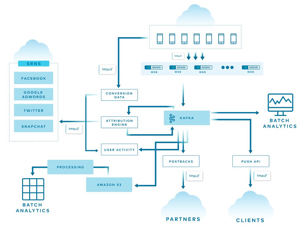
The diagram above is a simple overview of AppsFlyer’s architecture, and each line represents a different flow in the system. Some of the data is used, replicated, and enriched, while other data is stored in various databases for attribution, batch analytics, and more. At the end of the funnel are two services that consume all the data from the end-of-the-line Kafka clusters and store it into S3 using an in-house streaming service and Pinterest Secor.
All of this is translated into more than 1 million incoming HTTP requests per second and 150+ billion events per day spread across more than 20 Kafka clusters.
Before going into more detail, let’s first go over some basic Kafka terms and concepts.
Kafka basics
Kafka is used for building real-time data pipelines and event streaming applications. An offset is a simple integer that Kafka uses to identify a position in the log. Lag is simply the delta between the last produced message and the last consumer’s committed offset. Today, offsets are stored in a special topic called __consumer_offsets. Prior to version 0.9, Kafka used to save offsets in ZooKeeper itself.
In the Offset Management proposal document, the Kafka Core team describes this implementation as a kind of “marriage of convenience” since Kafka is already heavily dependent on ZooKeeper for various purposes like cluster membership, elections, and configuration storage. Now, there are few services that implement their own offset management and store it in ZooKeeper itself. A good example of this is Pinterest Secor, as mentioned earlier.
There is, however, a flaw with this implementation: The problems associated with it become more apparent when you use thousands of partitions and hundreds of consumers. ZooKeeper is not built to serve high-write load such as offset storage. Therefore, the Kafka Core team decided to create a new special topic called __consumer_offsets. This topic allows offset management to be consistent, fault tolerant, and partitioned across the Kafka cluster itself. In fact, one of the most anticipated Kafka Improvement Proposals (KIPs) is KIP-500, which will remove the dependency on ZooKeeper completely. After KIP-500 is implemented, Kafka will manage its own metadata internally in a more scalable and robust way, and it will omit the option to use ZooKeeper-based consumers.
How does offset storage work?

When the group coordinator—a broker that is selected to manage the state of a given consumer group—receives an OffsetCommitRequest by the application, it appends the request to the __consumer_offsets topic, which is then replicated to other Kafka brokers in the cluster based on the offsets.topic.replication.factor config parameter. This specifies the replication factor of the offset topic and affects the amount of brokers the offset commit will be replicated to.
The offset commit can be controlled from the broker configuration. You can set the offsets.commit.required.acks, which stands for the number of acknowledgments that are required before the offset commit can be accepted, as well as offsets.commit.timeout.ms, which defaults to five seconds.
The simplest way to check the offsets and lag of a given consumer group is by using the CLI tools provided with Kafka.

In the diagram above, you can see the details on a consumer group called my-group. The command output shows the details per partition within the topic. Two main columns that are worth mentioning are the CURRENT-OFFSET, which is the current max offset of the consumer on a given partition, and the LOG-END-OFFSET, which is the offset of the latest message in the partition.
Why does lag matter?
Why does lag matter and why does it need to be treated differently than other metrics in the system?
Lag is a key performance indicator (KPI) for Kafka. When building an event streaming platform, the consumer group lag is one of the crucial metrics to monitor.
As mentioned earlier, when an application consumes messages from Kafka, it commits its offset in order to keep its position in the partition. When a consumer gets stuck for any reason—for example, an error, rebalance, or even a complete stop—it can resume from the last committed offset and continue from the same point in time.
Therefore, lag is the delta between the last committed message to the last produced message. In other words, lag indicates how far behind your application is in processing up-to-date information.
To make matters worse, remember that Kafka persistence is based on retention, meaning that if your lag persists, you will lose data at some point in time. The goal is to keep lag to a minimum.
What did we have?
A few years ago, when Kafka became a crucial piece of AppsFlyer’s infrastructure, we created a Clojure service called Kafka-Monitor. It was essentially a simple wrapper around the built-in Kafka CLI tools that were mentioned before, which parsed the values and sent it to our metrics stack. Although it worked fine, it was hard to maintain, error prone, and not scalable at all.
We also recognized that something was missing. Just imagine a situation where you get a PagerDuty alert on Kafka lag in the middle of the night. You barely wake up, open the laptop lid, and try to understand what’s going on in your system.

In such a scenario, the last thing that you want to do is to start debugging and calculating the lag, calculating the retention time, and figuring out what you should do next.
This information should already be as descriptive, clear, and actionable as possible. The fact that the lag is represented by a number means very little. Does a 40,000 message lag mean five seconds? Five minutes? Is there a risk of losing data because of retention?
This was the blindspot that needed to be addressed.
What did we want to achieve?
When planning for a better solution for lag monitoring, the following needs were defined for the new solution:
- Automation: We wouldn’t need to change config files and deploy the service every time a new consumer group that we want to monitor starts to consume from the cluster.
- Regex filter: We want the ability to control which consumer group to monitor based on a predefined regular expression (e.g., filter out test consumers, and the
console_consumers). - Support ZooKeeper consumers: We want a solution that will track both
__consumer_offsetsas well as ZooKeeper consumers. - Scalable: AppsFlyer scale continues to grow every single day. Thus, we need a solution that will scale and has a small footprint so we can deploy it for each cluster and scale it horizontally as needed.
From a metrics perspective, we wanted the ability to control and build our own calculations and alerts because we use Kafka for different use cases and have different monitoring stacks. The raw metrics that we searched for included per-partition, per-consumer-group, and per-topic metrics. These metrics provide flexibility for lag monitoring and alerting, and help create lag monitoring that actually means something.
What options did we consider?
With those guidelines, we started to explore and test a few of the available solutions.
The prominent ones were:
Kafka Lag Exporter
Kafka Lag Exporter had native Kubernetes support and contained time-based lag monitoring out of the box. At the time, it was in beta and it didn’t fit our predefined guidelines.
Remora
Remora was created after Zalando spent some time using Burrow. It has Datadog and CloudWatch integration, and it’s a wrap around the Kafka consumer group command—which we already had.
Burrow
Burrow is an active LinkedIn project with more than 2,700 stars on GitHub. It has an active community, Gitter channel, great wiki page, and multiple extension projects. Burrow is battle tested and works in production at LinkedIn.
We chose Burrow because it answered all our needs, including tailor-made metrics calculations, providing enough flexibility to expose the metrics at different levels, and calculating lag time. At the current time, we are also considering Confluent Platform, because it provides many components that we would otherwise need to build and implement on our own. Confluent Platform also includes Confluent Control Center, which is another monitoring tool for Apache Kafka.
So, what is Burrow?
Burrow
Burrow is a monitoring solution for Kafka that provides consumer lag checking as a service. It monitors committed offsets for all consumers and calculates the status of those consumers on demand. The metrics are exposed via an HTTP endpoint.
Burrow also has configurable notifiers that can send status updates via email or HTTP if a partition status has changed based on predefined lag evaluation rules.
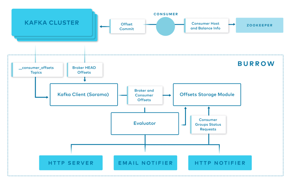
Burrow has a modular design and consists of the following components:
- Clusters/Consumers subsystem runs a Kafka client (Sarama) that periodically updates cluster information and consumes from the
__consumer_offsetstopic and from ZooKeeper. - Storage subsystem stores all of Burrow’s information. Burrow relies on ZooKeeper as well to store metadata for modules and provide locking between multiple copies of Burrow.
- Evaluator subsystem retrieves the information from the storage subsystem and calculates the status of a consumer group based on predefined lag evaluation rules.
- Notifier subsystem fetches the status of consumer groups and notifies via HTTP, email. or another predefined method.
- HTTP server exposes an HTTP endpoint for Burrow.
How do we use Burrow?
Burrow’s modular design and small footprint allow us to deploy it easily and efficiently to monitor a single Kafka cluster or a cluster group.

Above is an overview of how Burrow is deployed at AppsFlyer.
At AppsFlyer, Kafka clusters can be grouped logically and monitored together using Burrow. Using our in-house deployment system, we deploy three copies of Burrow in separate availability zones to monitor each cluster group. Each of them has a healer and autoscaler configured in our orchestration system based on a threshold.
The Burrow instances are connected to the same ZooKeeper ensemble. Each one of the Burrow instances exposes an HTTP endpoint where our metric stacks read or receive from, depending on if it’s Prometheus or Telegraf.
Burrow dashboards
Burrow exposes different sets of raw metrics, which gives us the flexibility to create tailor-made dashboards and alerts.

This dashboard enables us to visualize the lag by number of messages, the producer rate, the consumer rate, and a comparison between the two.
Another useful dashboard is the partition analysis dashboard.

With the previous solution, we couldn’t identify exactly which partitions were lagging behind, but with this dashboard, we can identify exactly which partition has the highest lag, correlate it with the partition leader, and potentially shed some light on the incident and find a misbehaving broker.
More importantly, we were able to achieve our end game: time-based metrics.
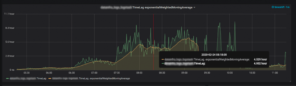
Time lag: How did we do it?
The most important metrics to collect are the last consumer message and the last produced message.
We know the lag per partition, per topic, and per consumer group. We also know the producer rate, which is our biggest assumption in the equation. We assume that the producer rate is stable—like a normal operating producer.
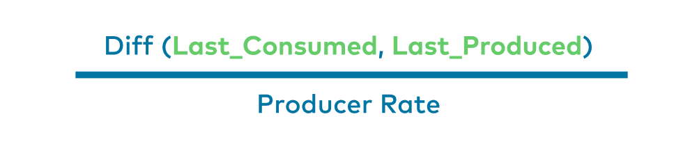
So if we will calculate the difference between the last consumed message and last produced message, and divide it by the producer rate, we will get the lag—in time units!
Here is a simple visual:

In the diagram above is a Kafka timeline. The producer produces one message a minute. At 12:00 a.m., the produced offset was 134. Ten minutes later at 12:10 a.m., the offset was 144. Ten minutes after that, it was 154, which is the current time.
While producing those messages, our consumer consumed messages at a given rate. Now, it just consumed the message that had the message offset of 134, which we already know was produced 20 minutes ago. It can then be assumed that our consumer is lagging 20 minutes behind the producer, as it just read a message that we produced 20 minutes ago. This is how we managed to get time-based lag metrics.
What’s next?
Consumer group lag is one of the crucial metrics to monitor in our system, and we addressed a major blindspot by developing actionable lag monitoring through a variety of metrics. But there’s still more to do.
Smart alerts
We want to create smarter alerts thresholds. As stated earlier, Kafka persistence is based on retention—meaning that if your lag is persistent, you will lose data at some point in time. If we have a time-based measure and the topic retention, we can trigger an alert before getting into a dangerous zone of a consumer that is not consumed fast enough and causes data loss because of the retention. To ensure this, we are using a Prometheus exporter to collect the retention (and other data as well), visualize it, and apply it in our alerting system.
Decoupling
As AppsFlyer continues to grow, and clusters load and traffic become greater, we will start decoupling “Burrow stacks” from monitoring the clusters group to monitoring a dedicated cluster. This can be performed easily because of the way that we implemented Burrow in our system. Once we split the configuration file in the dedicated Git repository and deploy, we’re good to go.
If you enjoyed reading this article and would like to learn more, you can check out my session at Kafka Summit for more details.
The post Apache Kafka Lag Monitoring For Human Beings appeared first on Leev's.
]]>The post How to collect Kafka configuration as metrics? appeared first on Leev's.
]]>Unlike other distrusted systems (i.e Aerospike), Kafka does not expose its configurations as metrics.
It makes sense in a way, config parameters and metrics are not the same, and most of the time you cannot represent configurations as metrics (strings).
But there are few useful configuration parameters that might be beneficial to collect in order to improve the visibility and alerting over Kafka in particular.
A good example might be log.retention.ms parameter per topic, which can be integrated into Kafka’s dashboards to extend its visibility, or to integrate it into an alerting query to create smarter alerts or automation based on topic retention.
So how can we do so?
“Kafka Configs Metrics Exporter”
I decided to create a Prometheus exporter to collect those metrics, using Kafka’s AdminClient to quickly pull all the config parameters that can be represented as metrics, expressly, can be converted into int .
After deploying the exporter and point it to your desired Kafka cluster, you will be able to query your metrics data source and create amazing graphs and alerts based on it!

The exporter and its documentation is available on GitHub
↧ ↧ ↧
https://github.com/EladLeev/kafka-config-metrics
The post How to collect Kafka configuration as metrics? appeared first on Leev's.
]]>