1. Introduction and System Overview

Accurate positioning and orientation are fundamental to producing high-quality LiDAR point clouds and their deliverables in mobile and aerial mapping. Traditional single-antenna GNSS/INS configurations often struggle in environments with limited satellite visibility, resulting in degraded heading accuracy and positional drift. The use of a dual-antenna GNSS system directly addresses these challenges by providing stable, motion-independent heading and faster recovery from GNSS interruptions. This configuration ensures consistent data quality and reliability, even in dense or obstructed mapping environments.

This case study evaluates the performance of the Inertial Labs RESEPI GEN-II – a next-generation mobile mapping platform integrating a Dual Antenna INS-D and XT-32M2X LiDAR – to demonstrate its capability in achieving high-precision results under challenging GNSS conditions. Conducted in Paeonian Springs, Virginia, the study highlights how the dual-antenna configuration enhances trajectory accuracy, improves LiDAR point cloud consistency, and minimizes drift when compared to single-antenna setups. The results confirm that RESEPI GEN-II provides robust and repeatable performance for professional mobile mapping applications where reliability and precision are critical.

Dual Antenna GNSS in RESEPI

In our last paper, we have discussed the impact of the IMU as part of the system and its effect on the accuracy of point clouds [1] and their deliverables. Let’s take a look at Figure 1, which shows just some of the factors that affect the accuracy of the acquired data. As you can see, there are many, and it is not only the accuracy of the IMU that affects the point clouds.

In this context, the choice between single or dual GNSS antennas becomes an important decision. The question may immediately arise: why pay more for a dual antenna system – doesn’t single antenna work just as well? Let’s consider the facts:

• A single GNSS-antenna cannot independently determine the heading of an object at rest – it requires motion and data from an inertial navigation system (INS). A dual-antenna system allows you to calculate heading directly, regardless of speed, by measuring the phase of the signal between the two antennas. This is especially important for precise orientation of the LiDAR scanner when starting, maneuvering or stopping.
• Dual GNSS in conjunction with the INS provides a more stable and accurate platform orientation measurement (pitch, roll, heading). This reduces the dependence on inertial measurement errors and reduces drift accumulation in the INS, especially in conditions with variable driving dynamics.
• In difficult conditions – near buildings, trees or other obstacles – the presence of two antennas helps to recover heading and orientation faster after GNSS signal loss, which is especially important for MMS (mobile mapping systems). Even in short-term shadows, the system can continue to correctly determine the platform’s orientation.
• With two GNSS antennas, it is easier and often times more accurate to calibrate offsets between GNSS, INS and LiDAR. This reduces point cloud alignment errors, reduces artifacts, and makes the point cloud more geometrically accurate.

 

Although a single GNSS antenna system may be cheaper, dual GNSS provides significantly higher orientation accuracy, which is critical for mobile LiDAR mapping. This is especially true for tasks that require centimeter accuracy and consistent data quality, such as engineering surveys, cadastral surveying, and high-precision mapping in complex urban environments.

Just for such tasks, Inertial Labs engineers have developed a dual-antenna system for MMS data acquisition as well as aerial mapping.

RESEPI GEN-II with XT-32M2X LiDAR

Experience superior aerial and mobile mapping with the RESEPI GEN-II, featuring the advanced XT-32M2X LiDAR (Figure 2). This system incorporates a lighter and longer-range version of the XT-32 scanner, enabling longer flights and higher operating altitudes (AGL) [2]. With an expanded vertical field of view (FOV), it’s ideal for efficiently surveying extensive regions, even those with dense vegetation. The RESEPI GEN-II stands out for its best-in-class data accuracy, extended detection capabilities, high point density, and overall adaptability.

The RESEPI GEN-II is an advanced, next-gen sensor-fusion platform built for high-accuracy remote sensing in aerial, mobile, and pedestrian (indoor, SLAM) applications. It leverages Inertial Labs’ Dual Antenna INS-D, featuring a Tactical Grade Kernel-210 IMU and an Extended Kalman Filter (EKF) for robust navigation both in real time and post-processed applications.

This system offers enhanced expandability, with capability for built-in software integrations via MAVLink and DJI’s Payload SDK (PSDK). Users benefit from new camera options with a wider FOV, faster shutter speeds, and higher resolution. Its field-swappable mounts ensure easy integration with platforms like the WISPR Ranger Pro 1100, Freefly Astro, Sony Airpeak S1, DJI M350 (or M400) and most importantly for this discussion – the dual antenna mobile mount from Inertial Labs.

The GEN-II’s powerful on-board computing module allows for real-time point cloud visualization (for quality control and fast decision making) and supports integration of external sensing modules, letting users synchronize additional cameras, LiDAR, or input aiding data from various sensors. This makes it a highly customizable and versatile plug-and-play hardware package, ideal for end-users and engineering firms. Some of the system specifications are shown below in Figure 3.

2. Mobile Mapping Study Description

To demonstrate the capabilities of the system, we organized a mission in a mobile configuration. Most suppliers sell results and performance specifications that in reality turn out to be only ideal-conditions which are almost never replicable for the end-user. Inertial Labs prides itself in not only making quality products but being a trustworthy partner that offers integrity and honesty.

A typical mobile mapping mission includes the following as an operating procedure for data acquisition:

1. 30 second to one-minute static alignment in ideal GNSS conditions (open sky);
2. 5 minutes of driving in ideal GNSS conditions where observable changes in heading, position, pitch and roll are experienced – prior to driving into mission area;
3. User proceeds to area of interest for mapping. This duration of time varies based on project. Depending on conditions of GNSS, consider including segments of coverage in areas of high-quality GNSS to ensure positional accuracy throughout the dataset.
4. 5 minutes of driving in ideal GNSS conditions where observable changes in heading, position, pitch and roll are experienced – after driving out of mission area;
5. 30 second to one-minute static alignment in ideal GNSS conditions (open sky);

For this test, we spent only a few moments in quality GNSS coverage before proceeding into areas with dense tree cover. This was done intentionally to demonstrate the power of a less-than-optimal workflow to highlight the capabilities of the Kernel-210 Inertial Labs IMU with a dual antenna GNSS receiver inside the RESEPI GEN-II system.

Below is a brief description of the test that was performed:

Location: Paeonian Springs, Virginia, USA.

Terrain type: Paeonian Springs, Virginia, is characterized by gently rolling countryside, representing a rural-suburban transition area within the broader Virginia Hunt Country. It features a mix of wooded areas and open farmlands, as shown in in Figure 4.

Land Features: The presence of tall trees with dense crowns (Figure 5) coupled with open skies.

Mission Purpose: To showcase the performance of RESEPI GEN-II as a mobile mapping solution when standard operating procedures are not followed and in effect demonstrate to customers what performance can be achieved even in less-than-ideal conditions.

Equipment used: For this project, we deployed a standard set of RESEPI available equipment as follows:

Mobile Platform: A pickup truck served as the mobile platform, specially adapted for the stable mounting of geospatial equipment.

Remote Sensing System (Payload): The core data acquisition system was the RESEPI GEN-II with XT-32M2X LiDAR. This advanced LiDAR configuration, featuring the lighter XT-32M2X scanner with an extended detection range, was crucial for capturing high-accuracy and dense point clouds, vital for detailed mapping requirements.

Navigation Equipment: The RESEPI GEN-II system integrates Inertial Labs’ Dual Antenna Inertial Navigation System (INS-D), which includes a Tactical Grade Kernel-210 IMU and a dual antenna NovAtel OEM7720 GNSS receiver.

Dual-Antenna Mobile Mount: To optimize the performance of the dual-antenna INS on the previously mentioned pickup truck, a customized mount was installed (Figure 6). This ensured precise spatial placement and stability for the GNSS antennas. NovAtel Vexxis 802L multiband GNSS antennas were used.

Software: Inertial Labs’ PCMasterPro and LiDAR360 from Green Valley International.

Ground Control Points: Both control point and check points were gathered using differentially processed base data from an Emlid RS2+ recording static sessions with a minimum of 15 minutes each logged at a data rate of 20Hz.

In the next section we will look at critical portions of the data collection process.

3. Data Capture for Study in PCMasterPro

Using Real Time Streaming into PCMasterPro as Quality Control Tool

An indispensable feature of RESEPI GEN-II is the support of real-time data capture and transmission. Previously, the user organized a mission, then processed the data after. This would have been the users’ first opportunity to get a look at the point cloud. Although many tools exist to verify successful operation of the payload, nothing beats being able to look at a 3D representation of the environment you are scanning in real time to know for certain that capture is happening as expected. The ability to track data recording in real time will save the user a lot of time, and here’s why:

• Coverage assessment: You can see immediately, whether you’ve covered all the area you need to cover, exposing if there are any data gaps or “holes” in the point cloud that may require revisiting.
• Save time and resources: Instead of collecting data all day and then finding errors only after uploading and post-processing in the office, you can fix them on the spot before leaving the job site. This significantly reduces project turnaround time and reduces the cost due to repeat missions.
• On-site decision making: If you see that the data quality is excellent, you can complete the mission earlier or, conversely, decide it’s worth collecting more data in a certain area because time permits.
• Confidence in the outcome: When you see real-time data, you can be confident that the system is working correctly and collecting exactly what you need.
• Minimize risks: Continuous monitoring helps you avoid costly errors that can occur due to misconfigured equipment or external factors.
• Quickly detect anomalies: Unusual readings or abnormalities are immediately apparent, allowing you to immediately investigate the cause.

In essence, real-time data recording and visualizing is like an airplane dashboard for a pilot: it gives you all the information you need right now so you can make informed decisions, avoid errors, and do your job as efficiently as possible.

In PCMasterPro, to monitor and visualize real-time point clouds, simply click on the menu “Data Streaming” -> “Settings”. The window shown on the Figure 7.

You can learn more about how to set up Point Cloud Streaming by clicking here [3].
Next, we will cover a very important topic which is critical for accuracy and precision both for real-time and post, the importance of lever arms and how to use them properly.

Using Fixed versus Estimated Lever Arms versus for Optimal Accuracy and Precision

In our previous articles, we have repeatedly mentioned that PCMasterPro uses NovAtel Inertial Explorer (IE) for post-processing GNSS+IMU data. But we have not previously considered in detail the features of its operation, particularly the Lever Arm Definition. PCMasterPro (thanks to IE) has functionality that allows you to estimate (calibrate) levers – that is, the displacement vector between the GNSS antenna(s) and the IMU center. This procedure is called lever arm estimation.

How it works:

1. During post-processing (Forward/Reverse/Combined), IE analyzes INS and GNSS data using the differences between the expected and measured trajectory.
2. Based on the dynamics of movement (especially in 3D), IE can estimate the antenna displacement vector, minimizing errors between the INS and GNSS position.

Ideal conditions for a good estimate:

1. There should be a variety of movements (not only a straight line): turns, tilts, accelerations, even static conditions for biases to be estimated at beginning and end.
2. Antenna(s) are placed in locations where they are not hidden underneath structures that block line of sight with satellites.
3. During the data capture, it is important for there to be quality GNSS coverage during the entire operation. Low exposure of satellites (tunnels, narrow canyons) or satellite visibility from low elevation angles result in poor estimates of antenna positions.

 

PCMasterPro assumes that the GNSS antenna(s) are fixed relative to the IMU. If it is moving (e.g. on a flexible bracket), the result will be inaccurate. If all conditions are met, the software will automatically estimate the offset to within an estimate accuracy of 1 mm.

But there is another, more reliable approach especially for mobile environments where areas with poor satellite coverage may exist and be common. If the offsets are already known whether by measurement or by CAD drawing, you can process manually assigning these as the desired values to use during point cloud creation. In cases of poor GNSS environments you will always end up with a more reliable and accurate solution if you do this, and here’s why:

1. Maximum reliability: if measured accurately, it is “ground truth”, independent of the algorithm.
2. More predictable result: there is no risk that the program will make a mistake due to lack of maneuvers or noise.
3. Less dependent on the trajectory: even if the trajectory is simple or straight, the values will still be correct.

 

Of course, not everyone will be able to measure an arm manually with an accuracy of 1 mm without having special equipment. Therefore, we have given recommendations on how to get the best results in PCMasterPro by combining automatic estimation and manual input of lever arms, as follows:

• If in environment with perfect conditions:
  • Use dual antenna processing, sampling rate of differential solution = 20Hz, Lever Arm Refinement = auto;
• If in environment with non-perfect conditions:
  • Use dual antenna processing, sampling rate of differential solution = 1Hz, Lever Arm Refinement = off;
  • Forced lever arm values must be KNOWN. For best results, perform initial drive test in perfect environment, use refine lever arm features to determine the exact lever arm, and then use these values to manual input lever arm in environments that are not good.
    • Alternatively, if using our mobile mount hardware, we provide exact lever arm values computed from CAD software (see below).

 

Using our proprietary mount (Figure 8), the user does not need to perform an initial drive test because we have already computed results perfectly from our design software. The user simply specifies the offsets in PCMasterPro and the software does the rest for you.

Manual input of levers is more accurate and reliable, especially if you are building a map or model where high absolute accuracy is important (for example, centimeter accuracy of a point cloud).

Auto-estimation is reasonable to use for constantly good GNSS conditions, testing, preliminary mobile sessions, or if equipment is not available for measurements. However, if you find yourself in a situation where these are untrue for your mission taking advantage of alternative methods is helpful, specifically forcing known and computed lever arm values into the pre-processing engine. Configuring these values during pre-processing and even during data collection results in faster processing, accurate real-time point clouds (and data visualized within PCMasterPro), and more reliably consistent deliverables.

In the next section, we will look at the RESEPI data pre-processing workflow in our proprietary PCMasterPro software for this case study.

4. Dual Antenna Pre-Processing in PCMasterPro and Point Cloud Creation

Returning to our mission, after collecting the data, we processed it in our proprietary PCMasterPro software. The processing procedure is very simple and does not require any significant competencies. Below we provide detailed instructions on how to process dual-antenna GNSS projects in PCMasterPro:

1. Copy the raw project data to your computer.
2. Open them by double-clicking on “ppk.pcmp” or directly in PCMasterPro via the menu “File” -> “Open Project”.
3. The program will unpack the archives and display a window with data entry for the base station and antenna offsets, as shown in Figure 9. Note that we selected the 1Hz frequency and manually set the antenna offsets that were shown in Figure 8. This was done intentionally because the GNSS quality in the environment driven was not perfect and prone to error to do poor satellite visibility on tree-covered rural roads.

4. After entering the parameters, click “OK”. This will start the processing, which no longer requires user intervention (Figure 10)

5. After completing the data processing, we obtained the point cloud shown in Figure 11.

6. Select the portions of the path you would like to output the point cloud for.
7. We now exported this point cloud for further processing to follow a typical MMS workflow in LIDAR360 from GreenValley [4].

 

Next, we look at the post-processing procedure for a MMS workflow and resulting accuracy assessments in LiDAR360.

5. MMS Post-Processing in LiDAR360 for Alignment and Adjustment with Ground Control

Due to the complex nature of GNSS conditions associated with mobile mapping, most state and local entities encourage and even require the use of ground control for not only accuracy assessment but correction. This helps ensure reliability and proper alignment with local defined geographic landmarks. LiDAR360 from GreenValley contains some helpful tools where we will show what accuracy is achieved in a less-than-optimal environment. In this section, we will walk through a typical MMS workflow to assess accuracy of classified ground points. First, we begin by importing the point cloud. In LiDAR360, this can be done in several ways:

1. Use the Quick Access menu in the upper-left corner, as shown in Figure 12a.
2. As shown in Figure 12b, click on the “File” button and then click on “Add Data” in the window that opens.

A dialogue box will pop up to specify the path to the .las (.laz) file.

After selecting the file, the program will display the header information of the .las (.laz) file in the window shown in Figure 13 (a, b, c).

In the additional tabs, you can select the attributes that will be read from the .las (.laz) file, subsample them, or reproject the point cloud to another coordinate system. All attributes are selected by default, there is no subsampling, and the coordinate system is automatically selected according to the point cloud georeferenced. We’ll leave all these options at their defaults. To load the point cloud, click on “Apply”.

After importing the main window of the program has the view shown in Figure 14.

In a typical workflow it is now necessary to subsample the point cloud for faster data processing. To do this, click “Other Point Cloud Tools” -> “Subsampling”, as shown in Figure 15. For the demonstration we used default settings.

The standard next step is to filter the point cloud for noise. To do this, click “Other Point Cloud Tools” -> “Noise Filter” on the “Tools” tab. For the demonstration we also used default settings, as shown in Figure 16. But in your case, you may need to tweak the parameters to achieve the best results.

Once the filtering is complete, go to the “Classification” tab and click on “Classify Ground Points”. The window shown in Figure 17 will open.

We also used the default settings, but the user should adjust them as needed to get the best results. Then, select the preset according to the type of terrain, in our case it is a slightly hilly terrain with vegetation. After classification we return to the “Tools” panel, click ‘Extract’ -> “Extract By Class” and specify the class “Ground”. Then we will work only with the ground-point cloud. The result is shown in Figure 18.

Next, control points were brought into the project. On the “Preprocessing” tab click on “3D Control Point Report”. In the opened window select “Check Type” – “Elevation” and click “OK”. Click on the icon to open a file with GCPs. The point cloud was de-biased with the control points and then analyzed for errors. After importing and adjusting the points to align them to the coordinate system of the project, set the required fields according to the order of data in the file and click run “Control Point Report”. Results are shown below in Figure 19.

It is important to note P7 stands out as an outlier from the dataset that is being analyzed. Multi-constellation/frequency differential GNSS solutions, especially with baselines like ours of less than a kilometer have well known accuracies of sub 3cm. For our control points to have any alignment error of -7.2cm is noteworthy. This point typically would be collected again or analyzed further, however one of the main purposes of this case study is to highlight the powerful alignment tools within LiDAR360. For this purpose, it was kept and used for the duration of the case study.

With all points considered, the average magnitude is 3.1 cm and the RMSE error is 3.7 cm. These results alone are not bad results, but in a traditional MMS workflow the use of control points to correct the data are often required, and will see what happens when we do the same. For this we will use the utility “Elevation Adjustment”. To use this utility, we need to export “Control Point Report”. For correction we will use 5 points out of 10, and in our case, we have chosen 1, 3, 5, 7, 9.

Now we will correct the error using the automatic alignment in the “Preprocessing” -> “Transformations” -> “Elevation Adjustment” tab. In the window that opens, specify the path to our new report file, as shown in Figure 20.

Click “OK” and wait for the automatic elevation correction process to complete. Next, we will check the results using the “Control Point Report”. The results are shown in Figure 21.

As you can see, the result is an average magnitude = 1.5 cm, and RMSE = 2.2 cm. Excellent accuracy in difficult GNSS signal conditions, and very good error compensation.

By leveraging our cutting-edge hardware, including the RESEPI GEN-II with XT-32M2X LiDAR and its integrated Inertial Labs’ Dual Antenna INS-D, combined with sophisticated processing software, we achieved remarkable precision in our data. A summary of the results can be seen below in Figure 22.

This level of accuracy, was attained without incurring excessive labor costs or requiring extensive manual intervention, highlights our commitment to best-in-class solutions and translates directly into superior, efficient, and highly reliable results for our clients.

6. Conclusion and Discussion

This study demonstrated the practical performance and reliability of the RESEPI GEN-II with XT-32M2X LiDAR, equipped with the Inertial Labs Dual Antenna INS-D, in a real-world mobile mapping scenario under less-than-ideal GNSS conditions. The results clearly highlight the advantages of a dual-antenna integration, robust IMU performance, and intelligent software processing within PCMasterPro and LiDAR360.

Despite intentionally minimizing ideal GNSS initialization and exposing the system to dense vegetation and intermittent satellite visibility, the system achieved highly accurate and consistent results. Before ground control alignment, the system produced an average magnitude error of 3.1 cm and an RMSE of 3.7 cm. Following elevation adjustment and automated correction within LiDAR360, accuracies improved significantly to 1.5 cm / 2.2 cm. These results represent a 52% improvement in average magnitude and over 40% improvement in RMSE, highlighting the effectiveness of the integrated hardware–software workflow.

Governing bodies such as: USGS, ASPRS, FHWA, DOT, lay out the requirements by which most federal, state, and project-specific jobs are defined by. These requirements include many things specifying vertical accuracy, horizontal accuracy, control spacing for ground points, and many other operational procedures to ensure consistency and accuracy across the many public and private entities that utilize such standards. Most mobile projects require a vertical accuracy of less than 5cm RMSE and a horizontal accuracy that is twice that, being less than 10cm RMSE. California and New York have some of the tightest requirements where many jobs will have vertical accuracy requirements of even 2cm or less. For these jobs control spacings are typically tight (every few hundred meters) where corrections are not just expected, but required, to ensure any and all drift or GNSS related errors are corrected for.

The RESEPI system, as shown from this case study, even with a less-than-optimal workflow demonstrates capabilities that directly translate into practical solutions for problem spaces of: corridor mapping, bridge and pavement inspections, infrastructure management and even engineering design work.

In conclusion, this case study validates the RESEPI GEN-II platform as a highly capable and dependable mobile mapping solution that performs exceptionally well even outside ideal conditions. The combined use of dual-antenna GNSS, a tactical-grade IMU, and advanced software integration ensures centimeter-level precision, reduced field time, and streamlined project workflows. These results establish a strong foundation for future deployments in urban, forested, and otherwise GNSS-challenging environments—confirming Inertial Labs’ commitment to providing reliable, accurate, and field-ready geospatial solutions.

References

[1] “Deep Dive into RESEPI Accurate Data.” Inertial Labs, 25 Mar. 2025. Accessed 28 July 2025.
[2] “RESEPI GEN-II M2X-ILX.” RESEPI, 7 Mar. 2025.
[3] “Real Time Point Cloud Streaming.” RESEPI, 7 July 2025. Accessed 28 July 2025.
[4] “LiDAR360 Point Cloud & Images Post-Processing and Industry Applications Software – GreenValley International.” Greenvalleyintl.com, 2022.

The post Precision Mobile Mapping with RESEPI GEN-II Dual GNSS in Practice appeared first on RESEPI.

With climate change, the risk and intensity of flood and wildfire events have increased significantly. Here in the U.S., the Palisades fire in Los Angeles made news earlier this year and other major global fires from this year alone include those in Israel/the West Bank, South Korea, the Amazon and the Arctic Circle.

The U.S.’s most deadly wildfire in over 100 years took place just two years ago, in August 2023, with the Lahaina fire on the island of Maui, Hawaii taking over 100 lives. It is also estimated that over 2,000 structures were destroyed, with overall losses initially projected to be in excess of $6 billion USD.

In this blog we’ll examine how the geospatial data and mapping consultancy firm Basemap Consulting has implemented LiDAR, camera, and PNT data from VIAVI’s Inertial Labs division and Hexagon | NovAtel to help rebuild communities after the Lahaina fire.

Mapping the Extent of the Damage

Following the fire, the pace of recovery has been, to an extent, limited by logistical, regulatory, and practical challenges. Hawaii’s isolation can mean that resources are limited or need to be imported, including building materials, labor, and specific skills.

Resources that can be deployed quickly are a plus and aerial and satellite images are now foundational tools for disaster planning and response. Notably, LiDAR and InSAR (interferometric synthetic aperture radar) are rapidly being adopted for post-event assessments.

One of the key challenges in rebuilding is that there is very little left in the hardest hit areas, meaning property boundaries are hard to identify and fresh surveys are an essential first step. Due to permitting and financing processes, surveying individual properties is not very efficient and is a significant cost burden.

Before the fire, drones were being discussed as a way to boost the efficiency of surveying. After the fire, they became a vital tool in defining the property boundaries, alongside physical features, terrain, structures, utilities, and trees.

The Capture

Capture began in late 2024, once the cleanup of debris in the area was nearly complete and permits for the flights were secured.

The first step was to divide the 1,500 acres (600 hectares) of interest into five subsites, which was undertaken via an imaging flight from a hill overlooking the affected area. Next, Basemap placed several standard aerial targets in each subsite. New and recently repainted street monuments were also repurposed to serve as additional aerial targets.

Tying these images back to precise locations is essential. For this, GNSS data was taken from a newly created reference station on a nearby hill. From this, Basemap augmented this with a portable GNSS base station.

These observation files were then used by Basemap in a post-processed kinematic (PPK) combined with an inertial measurement unit (IMU) step using VIAVI’s Inertial Labs’ PCMasterPro software. This software features Hexagon | NovAtel’s Waypoint Inertial Explorer and provides the spatial fidelity needed by the images and LiDAR point clouds to meet surveying and engineering specifications.

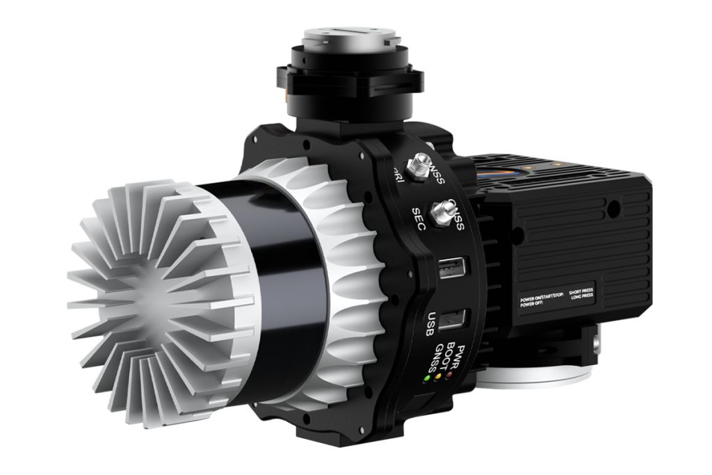
To achieve this, Basemap used a RESEPI Lite (Remote Sensing Payload Instrument) from Inertial Labs, a VIAVI Solutions Company. This is a combined single-antenna GNSS-aided inertial navigation system with datalogger (with this provided by the OEM7 receiver from Hexagon │ NovAtel), LiDAR, camera, and communications system. For this system, a Kalman filter is also applied to the output before synchronizing with GNSS data.

This Waypoint IE software is fully integrated with third-party IMU data and couples GNSS information from up to 32 bases with inertial data to deliver precise location information even with lower-grade inertial sensors.

Finally, Basemap also deployed a Sony A5100 24MP OEM vision camera and XT32 LiDAR system.

Ensuring the Tech Stack is Right

There are three key considerations when creating the technical composition of a drone reality capture system. The first is the laser, with the choice of LiDAR capabilities dictated by the end purpose for which it’s being used. The second consideration is the camera and many drone LiDAR systems – including VIAVI’s Inertial Labs’ offerings – integrate an RGB camera to collect both LiDAR points and high-resolution imagery simultaneously. The photos produced by this can be used not only for traditional photogrammetry, but also for colorizing the LiDAR’s point cloud.

It’s important to note that each sensor’s stated performance is for very specific conditions, meaning consideration in their selection is important to meet these conditions.

The third and most fundamental consideration is the system core, with its onboard processing/algorithms and its PNT technology. Without high-quality PNT systems, it will be impossible to generate the vital laser point clouds or color images, as these require precise information on both the location and orientation of the system.

As such, RESEPI has been created to provide a high-quality core first and is bundled with a range of sensors to meet the multiple needs of different applications, with the technology available in a broad range of payloads and focusing on applications where size, weight, and power (SWaP) criteria are critical to success.

Rebuilding

Lahaina has been a significant Pacific trading hub, the birthplace of kings, and the seat of the Hawaiian Kingdom during the 1800s. It has been, until the fire, seen as a vision of beauty and tranquility. Rebuilding the community is vital, but the pace of this is handicapped by the challenges of being a remote island with few surveyors, and reduced access to building materials, labor, and skills.

The approach taken by Basemap Consulting highlights the important role that using drone-based imaging and LiDAR mapped precisely using PNT networks can play in the rebuilding of a community after a natural disaster.

Using this combination of imaging and LiDAR capture flights, Basemap was able to provide local surveyors and developers with a precise and comprehensive spatial foundation alongside data on terrain, and any existing features that would prove useful for engineering design.

According to Basemap Consulting’s CEO, Daniel Windham, photogrammetric and LiDAR drone capture reduces the project’s work by between 50 and 80%, versus traditional surveying methods, and most features can be heads-up drafted from images and LiDAR point clouds.

Contacts

William Dillingham
Senior Manager, Product Marketing
Inertial Labs Inc, a VIAVI Solutions company

E-mail: [email protected]

The post The Crucial Role of PNT and Reality Capture Technologies in Rebuilding Following a Natural Disaster appeared first on RESEPI.

The National Defense Authorization Act (NDAA) is a cornerstone of U.S. defense policy. It defines not only the defense budget but also the standards for secure, transparent technology sourcing. Section 889 of the Act restricts the use of electronic components from unverified or high-risk suppliers, ensuring that every element in a compliant system comes from trusted and certified sources. Over time, NDAA compliance has become more than just a regulation — it is now a global benchmark for technological transparency and reliability, recognized by both government and commercial users.

Why NDAA Compliance Matters for Drone Payloads

In unmanned aerial systems, security is every bit as critical as performance. Payloads equipped with LiDAR, cameras, and inertial sensors collect large volumes of geospatial and visual data used in mapping, inspection, and defense operations. If a single component is not verified, it can compromise data integrity and limit where the system can be deployed. For system integrators and end users, NDAA compliance means peace of mind — knowing that every part of the payload meets the highest standards of security, traceability, and long-term reliability. It allows organizations to deploy UAV-based solutions without restrictions, fully aligned with U.S. and international procurement requirements.

NDAA-Compliant Payloads by Inertial Labs

The RESEPI OUSTER OS1-64 REV7 LiDAR, is a fully NDAA-compliant payload and one of the most advanced systems developed by Inertial Labs. This lightweight, high-performance LiDAR supports multiple scanning modes and flexible workflows, giving operators full control over data precision, density, and efficiency. With its 45° vertical field of view and compact design, RESEPI enables professionals to capture more data in less time — ideal for aerial mapping and inspection missions where both accuracy and speed matter.

The RESEPI GEN-II OUSTER OS1-64 REV7 LiDAR builds on this success. Developed through years of engineering expertise and real-world testing, it delivers survey-grade results for aerial, mobile, and pedestrian applications. Its versatile architecture and intuitive workflow make it a favorite among professionals who value consistent, reliable data. Compliant with NDAA standards, RESEPI GEN-II combines performance, transparency, and trust in a single solution.

Developed in collaboration with Teledyne Geospatial, the EchoONE merges Teledyne’s advanced LiDAR and imaging systems with Inertial Labs’ IMU and INS technology. This lightweight, NDAA-compliant payload produces long-range, engineering-grade 3D point clouds in real time. Built entirely to NDAA standards, EchoONE ensures data security, operational reliability, and cost efficiency, giving operators a dependable solution across a wide range of industries.

Built on Trust

Every NDAA-compliant system from Inertial Labs reflects our commitment to security, transparency, and engineering excellence. Whether for defense, infrastructure, or commercial missions, our payloads provide the confidence that your technology is trusted, compliant, and ready for critical operations.

The post NDAA Compliance: Trust and Security in Every Flight appeared first on RESEPI.

Amidst the rapidly developing spatial analysis technologies, forestry is increasingly adopting mobile LiDAR solutions for forest inventory and monitoring. This paper presents a field case study evaluating timber volume using a handheld RESEPI Ultra LITE system, which integrates laser scanning, inertial navigation, and SLAM (Simultaneous Localization and Mapping) technologies. The research object was a forest plot at Bear’s Den, a popular hiking and nature observatory in Loudoun County, Virginia, which is characterized by complex terrain and a dense canopy, which complicates traditional GNSS (Global Navigation Satellite System) methods.

To obtain a point cloud, the collected data were processed in PCMasterPro using SLAM and fixed georeferencing techniques (GNSS+SLAM). This is a new technology from Inertial Labs that enables the acquisition of a georeferenced point cloud when surveying SLAM data. The point cloud was then post-processed in Lidar360 software by Green Valley International using the TLS Forest toolset, which enabled automatic tree segmentation and extraction of key measurement parameters, including DBH, height, and volume.

The presented approach demonstrated high efficiency, allowing accurate measurements to be taken in difficult-to-access areas without the need for markers or manual measurements. The results obtained confirm the potential of GNSS+SLAM-LiDAR technology as a reliable tool for operational and sustainable forest resource management.

Introduction

The modern forestry industry faces a growing need for accurate, fast, and efficient inventory [1]. Tracking changes in forest stands, assessing biomass, monitoring logging, and regeneration require detailed and reliable information. Traditional methods, based on visual observations and point measurements, consume a vast amount of time, especially over large areas.

LiDAR (Light Detection and Ranging) is a technology that can radically change the approach to forest monitoring [2]. In recent years, mobile handheld or backpack LiDAR systems have attracted particular attention. Their main advantage is mobility and the ability to operate in complex conditions where unmanned aerial vehicles or terrestrial scanners are not feasible. In conjunction with hybrid GNSS+SLAM positioning technology, the use of modern analytics software for post-processing, such as Lidar360, provides a comprehensive solution that offers a qualitatively new level of data.

GNSS is the general term for satellite navigation systems, including GPS (USA), GLONASS (Russia), Galileo (Europe), and BeiDou (China). Many others are also used, but these are the major constellations. GNSS provides information about the absolute geographic coordinates of a location (latitude, longitude, altitude). SLAM is a technology that allows a device (camera or LiDAR) to simultaneously build a map of its environment and determine its location on that map. SLAM calculates the correct position of the sensor based on its motion and detection of surrounding objects.

GNSS provides georeferencing of the route’s start. When passing under tree crowns, the GNSS signal weakens, and SLAM continues to build a trajectory. After leaving the weak signal area, the GNSS again corrects SLAM’s trajectory. Without GNSS, error accumulation (drift) in the local coordinate system will be added to the SLAM map, which requires additional data processing for georeferencing.

Section 1. What is Handheld LiDAR and How Does it Work?

A handheld or backpack LiDAR is a mobile system combining a laser scanner and (optionally) a GNSS receiver and an inertial navigation system. The operator carries the system in their hands or on their back, walking through the area of interest, and simultaneously collects data that is then processed to obtain a three-dimensional point cloud.

This solution is particularly relevant for the forestry sector. Access to dense thickets, rugged terrain, and the inability to use vehicles or drones make mobile LiDAR systems indispensable. Scanning is performed in motion, without the need for tripods or the deployment of additional equipment, such as ground control points.

Let’s examine Figure 1, which displays a point cloud collected in a forest area using a handheld LiDAR system. As can be seen, this area has uneven and rocky terrain, which creates difficulties for vehicle movement and the deployment of TLS. In this case, a handheld scanner is a valuable solution. Unlike stationary TLS scanners, handheld LiDAR offers flexibility and mobility, allowing for easy navigation around obstacles and capturing the structure of undergrowth and trunks from different angles, thereby minimizing blind spots. Such data is critical for inventory tasks – from assessing tree diameter and height to biomass modeling and estimating timber volume. Thanks to the combination of compactness, accuracy, and the ability to operate in challenging conditions, handheld LiDAR is becoming a primary tool for modern forest mensuration, particularly in remote or inaccessible areas.

Figure 1. Point cloud obtained using handheld LiDAR.

SLAM technology plays a key role in the operation of handheld LiDAR systems, especially in conditions where GNSS is unavailable or unstable [3]. SLAM enables the construction of a map of the environment while simultaneously determining the sensor’s position in space without relying on external navigation. However, one of the main drawbacks of SLAM is the accumulation of errors (drift) – over time, the system can gradually lose positioning accuracy. This is particularly noticeable during long journeys without loop closure, when the device fails to return to a previously scanned area and therefore cannot correct its trajectory. This results in data displacement, which affects the geometric accuracy of the entire scene.

GNSS problems in forests should also not be underestimated. In dense stands, satellite signals are often blocked or reflected multiple times by the canopy, leading to significant positioning errors, especially when using standard GPS receivers without correction [4]. Even high-precision geodetic GNSS receivers lose effectiveness in forests if vegetation density exceeds a certain threshold. In such conditions, combining SLAM and GNSS becomes an optimal solution: GNSS provides absolute positioning, while SLAM ensures continuity of movement and detail within each scene.

Section 2. GNSS+SLAM: The Key to Accuracy in Challenging Forest Environments.

As mentioned in the previous section, one of the primary challenges when working in the forest is the limited availability of GNSS signals due to the dense tree canopy. This makes it impossible to obtain accurate positioning solely based on satellite data. By combining SLAM with GNSS (where the satellite signal is still available), you can achieve stable and precise positioning even in the complete absence of a GNSS signal. In this case, the point cloud will be geo-tagged, which is not possible with the standard approach used in scanning SLAM, as it operates in local coordinates. Such a hybrid scheme is actively used in modern LiDAR solutions, such as RESEPI Ultra LITE from Inertial Labs (Figure 2). The system enables the reliable construction of the operator’s trajectory and produces a highly accurate, georeferenced point cloud, even in deep forest areas [5].

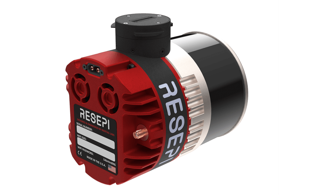
Figure 2. RESEPI ULTRA LITE.

Introducing the latest innovation from Inertial Labs, the lightest complete payload featuring both LiDAR and camera technology. Designed with the modern surveyor in mind, this solution offers unparalleled ease of use and versatility.

Key Features:

• Lightweight Design: Our lightest payload yet, ensuring ease of transport and deployment without compromising on performance.
• SnapFit Adapters: Experience seamless integration with various platforms (Freefly, WISPR, DJI, Sony, Mobile) through our quick plug-and-play SnapFit adapters, allowing for rapid dismounting and mounting.
• Cost-Effective: As the most affordable and comprehensive solution we’ve released, it provides exceptional value without sacrificing quality.
• Precision and Accuracy: Maintaining high data accuracy and precision has remained our priority and a promise to our customers. This product has undergone meticulous cycles of testing and refinement, utilizing proper time-stamping and calibration methods, to ensure we deliver unrivaled performance at the correct value.
• Multi-Mode Operations: Versatile in application, it supports aerial scanning, pedestrian hand-held SLAM (and GNSS+SLAM) operations, and vehicle-mounted mobile mapping, making it an all-in-one solution for diverse surveying needs.
• This product embodies Inertial Labs’ commitment to innovation and excellence, providing surveyors and key players in the 3D mapping space with a powerful tool that enhances efficiency and accuracy in their mapping projects.

For georeferencing, first, only SLAM data is processed. Then, PCMasterPro software analyzes all positions obtained using a GNSS receiver, selecting the most accurate ones. Using these positions, SLAM data is converted into a georeferenced coordinate system.

For this purpose, a GNSS antenna is installed on RESEPI, and data is recorded with satellites. After processing a geo-tagged point cloud, one is obtained; however, before processing, it is necessary to set the “Georeference Options” parameter to 2, as shown in Figure 3.

Figure 3. Processing parameters and geo-tagged point cloud in PCMaster Pro.

However, the point cloud itself is only the first step towards the desired solution; to obtain valuable information, it must be post-processed. For this, specialized software is used, which we will discuss in the next section.

Section 3. Case Study. Data Processing in Lidar360.

After the survey is completed, the data is processed in the Lidar360 software environment. Lidar360 is specialized software developed by GreenValley International for processing and analyzing laser scanning data [6]. It supports the processing of both terrestrial (TLS) and airborne (ALS) laser scanning data and is widely used in forest inventory, ecology, and geomonitoring. The program features a user-friendly graphical interface and a modular structure, with the main functions organized into toolboxes designed to perform specific types of analysis. Among them, the TLS Forest and ALS Forest Toolboxes are particularly valuable for forestry applications. TLS Forest is designed to work with dense point clouds obtained using terrestrial LiDAR. It allows you to segment trees automatically, estimate DBH, height, and calculate the volume of each tree. ALS Forest Toolbox, in turn, is designed to analyze airborne laser scanning data.

Both tools feature automated processing, making Lidar360 a powerful platform for forest analytics. Let’s examine a real-life example of utilizing RESEPI Ultra LITE and Lidar360 in forestry.

SUBSECTION. Case Study: Timber Volume Estimation Using RESEPI Ultra LITE with GNSS+SLAM in Bear’s Den, Virginia

As part of a pilot project to assess the volumetric characteristics of a forest stand in a remote forest area, a forest plot in the Bear’s Den area of ​​Loudoun County, Virginia, was surveyed [7]. The location is characterized by dense canopy cover, pronounced relief, and limited accessibility for traditional surveying methods. The main objective was to estimate the timber stock using a non-contact survey method.

Technology used:

The RESEPI Ultra LITE universal platform was used to collect spatial data. This allowed the operator to move freely around the site, recording the forest structure in 3D even in conditions of total GNSS eclipse under a dense canopy (Figure 4).

Figure 4. A patch of forest in the Bear’s Den area.

The survey covered an area of approximately 2.3 hectares, with a total mission duration of around 5 minutes and 30 seconds. The scanning trajectory was locally closed to minimize SLAM solution drift. The generated geo-tagged point cloud retained high density even in the lower tier, which is key for DBH analysis.

Data processing:

Point cloud processing was performed in the Lidar360 software environment, using the TLS Forest toolbox. The program provided automatic filtering of unnecessary objects, extraction of the ground surface, classification, and segmentation of individual trees, as illustrated in Figures 5 and 6.

Figure 5. Tree classification.

Figure 6. Segmented trees.

Based on trunk segmentation and height analysis, key taxation parameters were obtained, as shown in Figure 7.

Figure 7. Calculated DBH, trunk height, wood volume, and tree crown characteristics.

Results obtained:

As a result of processing, the following estimates were obtained:

• Average DBH (over a 0.5-hectare site): 32 cm
• Average tree height (over a 0.5-hectare site): 11 m
• Estimated wood volume (total over a 0.5-hectare site): 108 m³

The field test confirmed the high applicability of SLAM+GNSS-LiDAR in complex forest terrain conditions. Using RESEPI Ultra LITE in conjunction with Lidar360 made it possible to obtain accurate, geo-tagged spatial data without the need to install markers or measure points using GNSS equipment.

Conclusion

Modern forestry requires highly accurate, operational, and reproducible methods for collecting data on stand condition. Classic approaches, such as manual measurements of tree diameter and height, remain relevant. Still, they are labor-intensive and do not scale well, especially in hard-to-reach or GNSS-denied areas. In this regard, mobile laser scanning systems combining LiDAR, inertial navigation, and SLAM algorithms are becoming indispensable tools for forest mensuration and spatial analysis.

The case study discussed in this paper demonstrates the application of a handheld LiDAR system, RESEPI Ultra LITE, in a natural forest environment in the Bear’s Den area (Loudoun County, Virginia). The primary objective of the survey was to estimate timber volume under conditions where traditional GNSS positioning is challenging due to dense canopy and terrain. The use of SLAM ensured continuous navigation through the forest plot without the need for deploying ground markers or performing manual measurements.

The collected data was processed in PCMasterPro to get a geo-tagged point cloud, as well as Lidar360 – professional software for working with point clouds. The use of the TLS Forest toolbox enabled the automatic segmentation of trees, estimation of diameter at breast height (DBH), measurement of tree height, and calculation of timber volume.

This approach demonstrated high processing speed and sufficient accuracy for decision-making tasks, such as planning logistics operations or calculating carbon stocks. Thus, the combination of handheld LiDAR, SLAM navigation, and advanced post-processing in Lidar360 provides a practical solution for field inventory in real-world conditions. It combines mobility, accuracy, and automation – qualities necessary for sustainable forest management in the 21st century.

References

[1] Wulder, Michael A, et al. “The Role of LiDAR in Sustainable Forest Management.” The Forestry Chronicle, vol. 84, no. 6, 1 Dec. 2008, pp. 807–826

[2] “RESEPI – LiDAR Payload & SLAM Solutions.” RESEPI, 12 July 2024.

[3] Wikipedia Contributors. “Simultaneous Localization and Mapping.” Wikipedia, Wikimedia Foundation, 8 July 2019.

[4] Mendez, Maria. “What Are the Limitations of GNSS?” Inertial Labs, 2 Oct. 2024.

[5] “RESEPI Ultra LITE.” RESEPI, 18 Feb. 2025. Accessed 9 May 2025.

[6] “LiDAR360 Point Cloud & Images Post-Processing and Industry Applications Software – GreenValley International.” Greenvalleyintl.com, 2022. Accessed 8 May 2025.

[7] “Loudoun County, VA – Official Website | Official Website.”.

The post Efficient forest inventory management with RESEPI ULTRA LITE: GNSS+SLAM technologies and analysis in Lidar360 appeared first on RESEPI.

• Material type. Different materials reflect infrared radiation differently due to their distinct physical properties.
• Distance to the receiver. The further an object is from the LiDAR, the weaker the reflected signal will be.
• Angle of incidence. The greater the angle at which the laser beam strikes the surface, the lower the intensity of the reflected signal.
• Weather conditions. Rain, snow, and fog can weaken the laser beam and reduce the intensity of the reflected signal.
• Type of LiDAR. Different kinds of LiDAR (for example, pulsed and continuous) may have different formulas for calculating intensity. This also includes the wavelength of the emission—for instance, 905 nm or 1550 nm will be reflected differently from the same objects under identical conditions.
• Laser wavelength. Different wavelengths may interact with various materials in different ways [1].

From the first two points, it becomes clear that intensity information can help in identifying and classifying objects. This approach is not new and has been in practice for a long time. There are several interesting articles on the subject, for example [2] and [3]. The work [4] is also noteworthy.

Let’s delve a bit deeper into how this works. Below is a simplified formula for the received signal power (1) [4]:

                                                                                                                                    (1)

where  is received optical power [W],   is transmitted power [W], = receiver aperture diameter [m],  = effective target cross section [m²],   is the atmospheric transmission factor,  is the system transmission factor,   is range [m], and  is transmit beamwidth [rad].

The effective target cross section (or effective scattering area)   is a measure of how well the LiDAR detects an object. This parameter can be expressed as follows (2):

                                                                                                                                  (2)

where  is target reflectance at the laser wavelength, Ω = scattering solid angle [sr], and  is target area [m²].

If the target is large enough to cover the laser beam completely and reflects light uniformly in all directions (like a Lambertian surface), then the equation describing the LiDAR range can be written as follows (3):

                                                                                                                                  (3)

where  is the angle of incidence of the beam.

These formulas are simplified and do not account for all factors affecting LiDAR intensity. However, they can help understand the basic principles of LiDAR operation.

For illustration purposes, we conducted a simulation using equation (3) with the simplification of  =  . Some of the values, such as the receiver aperture diameter, might be unknown, so we did not aim to use exact figures for any specific LiDAR. Instead, we made certain assumptions to demonstrate the dependence of the detection range on intensity. The simulation result is shown in Figure 1— as can be seen, the higher the reflectivity coefficient, the greater the detection range.

Figure 1. Dependence of detection range on intensity.

For ρ = 0.1, the maximum range ≈ is 30 m. For ρ = 0.325, maximum range ≈ 54 m. For ρ = 0.55, the maximum range ≈ 70 m. For ρ = 0.775, maximum range ≈ 83 m. For ρ = 1, maximum range ≈ 94 m.

The threshold value corresponds to 1 nW, which is typical for highly sensitive APD photodiodes [5]. We also note that intensity values are often normalized to a specific scale, for example, from 0 to 1 or from 0 to 255. This is standard practice in LiDAR systems. Therefore, if you have observed intensity values within a positive range in software used for processing or visualizing point clouds, it means that they have been scaled according to the LiDAR manufacturer’s specifications, as shown in Figure 2.

Figure 2. Intensity value range scaled to the manufacturer’s specifications.

                Intensity information is crucial for reliable and high-quality classification, as it is not always possible to classify objects solely based on their geometric features. There are patents proposing the use of intensity for object detection in autonomous vehicles [6]. Intensity is also used for classifying agricultural land by usage type [7].

Thus, intensity provides additional information about the surface that is not available using other methods. This approach enables increased measurement accuracy and enhanced quality of results. Intensity can be applied in various fields and used to solve different tasks. In conclusion, LiDAR intensity is a crucial parameter that significantly impacts the quality and accuracy of data obtained using this technology.

References

[1] Mendez, Maria. “Why Have 905 and 1550 Nm Become the Standard for LiDARs?” Inertial Labs, 18 Dec. 2024, inertiallabs.com/why-have-905-and-1550-nm-become-the-standard-for-lidars/. Accessed 14 Feb. 2025.

[2] Liu, Yuee, et al. “Classification of Airborne LIDAR Intensity Data Using Statistical Analysis and Hough Transform with Application to Power Line Corridors.” 2009 Digital Image Computing: Techniques and Applications, 2009, pp. 462–467, https://doi.org/10.1109/dicta.2009.83. Accessed 14 Feb. 2025.

[3] Christophe Reymann, Simon Lacroix. Improving LiDAR Point Cloud Classification using Intensities and Multiple Echoes. IEEE/RSJ International Conference on Intelligent Robots and Systems (IROS 2015), Sep 2015, Hamburg, Germany. 7p. hal-01182604⟩

[4] Kashani, Alireza, et al. “A Review of LIDAR Radiometric Processing: From Ad Hoc Intensity Correction to Rigorous Radiometric Calibration.” Sensors, vol. 15, no. 11, 6 Nov. 2015, pp. 28099–28128, https://doi.org/10.3390/s151128099. Accessed 25 Aug. 2020.

[5] “Avalanche Photodiode.” Wikipedia, 17 Feb. 2021, en.wikipedia.org/wiki/Avalanche photodiode.

[6] “US10598791B2 – Object Detection Based on Lidar Intensity – Google Patents.” Google.com, 22 Oct. 2018, patents.google.com/patent/US10598791B2/en?oq=US10598791B2. Accessed 14 Feb. 2025.

[7] Mesas-Carrascosa, Francisco Javier, et al. “Combining LiDAR Intensity with Aerial Camera Data to Discriminate Agricultural Land Uses.” Computers and Electronics in Agriculture, vol. 84, June 2012, pp. 36–46, https://doi.org/10.1016/j.compag.2012.02.020. Accessed 14 Feb. 2025.

The post What is intensity, and what does it affect? appeared first on RESEPI.

Here are the sections that will be covered: Introduction to LiDAR, Differences between scanning patterns, and the Risley Prism Scanner.

Section 1. Introduction to LiDAR

Light Detection and Ranging (LiDAR) is a remote sensing technology that utilizes laser pulses to measure distances with remarkable accuracy. By emitting laser beams and analyzing their reflections from objects or surfaces, LiDAR systems create detailed three-dimensional maps of the environment. This technology has become a cornerstone in various industries, including geospatial mapping, autonomous vehicles, environmental monitoring, and construction.

LiDAR operates on the principle of time-of-flight (ToF), where the system calculates the distance to a target by measuring the time it takes for a laser pulse to travel to the object and back (Figure 1). This data is then processed to generate a point cloud—a collection of spatially referenced points that represent the scanned area or object in three dimensions.

Figure 1. Conditional demonstration of LiDAR operation.

LiDAR is renowned for its high precision and ability to capture data in various environmental conditions. Some of its defining characteristics include:

• Accuracy: LiDAR can measure distances with centimeter-level precision.
• Versatility: It performs effectively in diverse settings, from dense forests to urban landscapes.
• High Resolution: The resulting datasets provide rich detail, allowing for intricate analysis.
• Speed: LiDAR systems can scan large areas, significantly reducing surveying time compared to traditional methods.

LiDAR’s versatility has led to its adoption across numerous fields:

1. Geospatial Mapping: LiDAR is extensively used for creating high-resolution topographic and bathymetric maps.
2. Autonomous Vehicles: Self-driving cars rely on LiDAR for obstacle detection, navigation, and spatial awareness.
3. Environmental Monitoring: It helps in studying vegetation, monitoring coastal erosion, and tracking changes in ecosystems.
4. Construction and Infrastructure: LiDAR aids in site analysis, construction planning, and structural monitoring.
5. Archaeology: Researchers use LiDAR to uncover hidden structures and map historical sites.

Ongoing advancements in LiDAR technology aim to address these issues by developing more cost-effective, compact, and robust systems. LiDAR is a transformative technology that continues to redefine our ability to observe and interact with the world. As it evolves, its impact is expected to expand, unlocking new possibilities across a wide range of industries.

Section 2. Differences between scanning patterns

Various scanning patterns (or scan templates), such as circular, linear, and others, are used in LiDAR and other systems to obtain spatial data. The operation of the LiDAR deflection system determines a particular pattern. There are many options for deflection systems. Figure 2 illustrates a conventional LiDAR deflection system, comprising an emitter, a receiver, and a system of mirrors (or prisms) that deflect the beam [1].

Figure 2. LiDAR Deflection System.

Mirrors or prisms can have different shapes and sizes. Depending on their geometry, the laser’s trace on the ground will differ. We will consider this in more detail below. Depending on the tasks, different mirrors or prisms are selected, for example, as shown in Figure 3 [2]. This is due to the requirement to scan only certain areas or within a specific angle.

Figure 3. (a) Cube prism; (b) ball prism; (c) open face mirror; (d) spherical housing containing 45° mirror, and (e) pentaprism.

In addition to mechanical systems, there are microelectromechanical ones. Recently, they have been rapidly developing due to the growing demand for miniature lidars. In such devices, the deflection system consists of a miniature mirror suspended on a platform. The deflection is done by actuators, as shown in Figure 4 (a). In reality, such mirrors have the form shown in Figure 4 (b).

Figure 4. Structure of MEMS Deflection System.

Now, let’s consider how the shape and orientation of the mirrors (or prisms) affect the trace left by the beam, as shown in Figure 5 [3].

As we can see, different mirrors and prisms can form similar patterns, and at the same time, the same mirrors can create various patterns, depending on their geometric position.

Let’s take a look at Figure 6. The first pattern (on the left) is a zigzag (there is also a sine wave variant). Raster or Zigzag Scanning is used in ground systems and mobile platforms.

Figure 6.

The second option is a linear pattern (in the middle). Often used in airborne LiDAR systems and ground-based scanners.

The last pattern (on the right) is Rotary or Circular Scanning. It is used in scanners equipped with a rotating mirror or a rotating device.

Some LiDARs have a more complex pattern, which resembles a spirograph pattern, for example, as shown in Figure 7 [4].

Figure 7. The typical point cloud patterns of the Livox Avia over an extended period.

Such a pattern allows you to achieve a very high density of a point cloud without movement, i.e., in a static setting. Such a pattern is obtained by using the Risley Prism Scanner.

Section 3. The Risley Prism Scanner

The Risley Prism is an optical device used to control the direction of a laser beam or other optical beam by independently rotating two prisms relative to each other [5]. The prisms are typically wedge-shaped and oriented in a manner that allows them to be rotated around their optical axes (Figure 8).

Figure 8. The Risley Prizm.

Parametric equations of point coordinates on a plane can be expressed as follows:

Where R is the beam displacement relative to the starting point, ω₁ and ω₂ are the rotation speeds of the first and second prisms, respectively.

For clarity, we will model these equations and examine the results. Let R = 1, ω₁ = 10√2, ω₂ = 1. Time t 10, 100, 1000 seconds. The results are shown in Figure 9. As you can see, the longer the prisms rotate, the more the circle is filled.

Now, we change the rotation speeds: ω1 = 1 and ω₂ = -1. That is, the prisms rotate at the same speed, but in different directions. As a result, we get a straight line, as shown in Figure 10. Unlike the previous case, this pattern remains constant over time.

Figure 10. The rotation speed of the prisms is the same, but the direction of rotation is different.

With the same rotation speeds in one direction, we get a circle, as shown in Figure 11.

Figure 11. The rotation speeds are the same, and the directions are the same.

For the next experiment, we will maintain the same rotation direction but increase the speed of one of the prisms, ω₁ > ω₂. The result is shown in Figure 12.

Figure 12. The speed of one of the prisms is higher, and the direction of rotation is the same.

Thus, by varying the speed and direction of rotation of the prisms, it is possible to achieve completely different patterns without changing the mechanical system. All these subtleties fall on the shoulders of optical system developers, but now you know how it works.

References

[1] lidar. “Velocity Determination from Lidar Point Cloud | in the Scan.” In the Scan, 27 Nov. 2023, blog.lidarnews.com/velocity-determination-from-lidar-point-cloud/. Accessed 13 Jan. 2025.

[2] Marshall, Gerald F, and Glenn E Stutz. Handbook of Optical and Laser Scanning. CRC Press EBooks, Informa, 23 July 2004. Accessed 3 May 2023.

[3] Zhou, Hao, et al. “Analysis of Internal Angle Error of UAV LiDAR Based on Rotating Mirror Scanning.” Remote Sensing, vol. 14, no. 20, 20 Oct. 2022, pp. 5260–5260, https://doi.org/10.3390/rs14205260. Accessed 15 Aug. 2024.

[4] “RESEPI Livox AVIA.” RESEPI, lidarpayload.com/home/resepi-livox-avia/.

[5] Application Note Risley Prism Scanner. https://www.thorlabs.com/images/tabimages/Risley_Prism_Scanner_App_Note.pdf

Foundation, 20 Sept. 2018, en.wikipedia.org/wiki/Theoretical_gravity.

[9] Lefevre, Herve C. The Fiber-Optic Gyroscope, Third Edition. Artech House, 31 Jan. 2022.

[10] “GPS-Aided INS-FI Datasheet Revision 1.9 FOG IMU-BASED GPS-AIDED INERTIAL NAVIGATION SYSTEM INS-FI.” https://inertiallabs.com/wp-content/uploads/2025/01/INS-FI_Datasheet_rev-1.9_Jan_2025.pdf

The post The difference between scanning patterns appeared first on RESEPI.

Obstructions to navigable airspace are recurring at the US Air Force Joint Base Lewis-McChord (JBLM) Airfield. Over 90% of the wooded areas surrounding the runway consist of Douglas Fir trees that grow between 3 and 6 feet per year and can reach heights of over 250 feet, penetrating the imaginary approach-departure clearance surfaces.

JBLM is required to conduct airfield obstruction inspections at least once every five years to ensure safe and navigable airspace. According to 14 CFR Part 77, an obstruction to air navigation is defined as an object that exceeds the height of imaginary airspace control surfaces. To guarantee safe aircraft landing and takeoff, the approach-departure clearance surfaces must be kept clear of objects and maintain a glide angle of 50:1 extending out to 500 feet above the runway.

Due to local and state environmental protection laws, airfield management cannot indiscriminately cut and remove Douglas Fir trees. Instead, trees can only be removed after they have been rated, appraised, and marked by a professional forester and classified as an obstruction to airfield operations. With over 1,000 acres of forest extending north and south of McChord Airfield, identifying each tree penetrating the imaginary surfaces is extremely difficult.

In March 2025, a pilot project was organized by the Air Force 627th Civil Engineer Squadron (CES) at JBLM to test and evaluate the use of drone Lidar and cloud-enabled software to inspect 1,000 acres of trees to the north and south of McChord Airfield. Led by Stitch3D with support from Inertial Labs RESEPI, Freefly, and BaseMap, the project was a tremendous success. Using a Freefly Systems Astro (Blue-Certified Drone), RESEPI Lite OS1-64 (NDAA-compliant LIDAR), and Stitch3D cloud software, the project demonstrated the ability to capture and deliver high-quality point cloud data within a 48-hour mission window despite adverse weather conditions.

Project Description

Target Sites

• JBLM North, approximately 250 acres.
• JBLM South, approximately 685 acres.

Mission Window

• 48 Hours (acquisition to delivery and reporting).

Equipment and Software

• Drone: Freefly Astro
• Mapping Payload: Inertial Labs RESEPI Lite OS1 (64)
• Processing Software: Inertial Labs PCMasterPro, Stitch3D Cloud

Deliverable

• Lidar Point Cloud with Ground Classification in project-required coordinate systems.
• Topographic Contour is derived from a classified point cloud in project-required coordinate systems.

Evaluation Metrics

• Timeliness
• Accuracy
• Data Interoperability and Shareability
• Ease of Use

Project Execution

Day 1 Acquisition

Due to bad weather conditions, heavy and intermittent rain, and strong winds of up to 35 miles per hour, the project team chose to cover only the smaller North Site. Flights were executed with the following mission parameters.

• Flight AGL: 55 meters (180 feet)
• Flight Speed: 5.5 meters/second (~12 mph)
• Flight Line Overlap: 35%
• Total Flight Time: 2 Hours
• Validation Survey: RTK Ground Control

Day 2 Acquisition

While the weather was more favorable, the South Site was much larger and mostly covered by dense, tall trees, which blocked stable radio communication between the drone and the remote controller. The project team was forced to execute aggressive battery swaps and utilize three launch locations. Mission parameters were slightly adjusted as follows.

• Flight AGL: 65 meters (213 feet)
• Flight Speed: 8.0 meters/second (~18 mph)
• Flight Line Overlap: 35%
• Total Flight Time: 5 Hours
• Validation Survey: RTK Ground Control

Data Processing

On both days, the collected flight data were immediately processed post-mission. Raw RESEPI data processing was performed in Inertial Labs PCMasterPro. The output point clouds (1.75GB for North Site and 5.58GB for South Site in LAZ format) were then post-processed in Stitch3D cloud to produce ground classification and topographic contour.

Results

Robust assessment showed that the JBLM pilot project produced very high-quality data. Point cloud point density averaged 321 pts/sqm and 329 pts/sqm for the North Site and South Site, respectively. Vertical accuracy (RMSE) was 1.3cm for the North Site and 2.2cm for the South Site. This high level of data quality meets typical land survey standards and exceeds what is required for JBLM airfield tree obstruction detection and mapping.

Conclusion

Despite adverse weather conditions, this project completed the flight coverage of the target JBLM airfield’s North and South approaches in a significantly reduced mission window and delivered high-quality results. All output spatial datasets were made available to 627 CES and 62 OSS stakeholders through Stitch3D cloud in a secure web environment, eliminating interoperability bottlenecks caused by different software and access points.
Based on the success of this pilot project, 627 CES made a strong recommendation that drone Lidar surveys be included as a routine part of airfield inspection operations.

About RESEPI Lite OS1

Powered by Inertial Labs’ advanced INS technology, RESEPI Lite OS1 (64) is a robust, cost-effective, and platform-agnostic Drone LiDAR data collection solution for accuracy-focused survey and mapping professionals, with expanded capabilities for mobile mapping (MMS) and SLAM-enabled scanning in a GNSS-denied environment. Key System Specs are as follows.

• System Vertical Accuracy (5 m/s @ 50 m AGL): 3-5 cm
• Laser Vertical Resolution: 64 channels
• Laser Number of Returns: up to 2
• Laser Points Per Second: 2,621,440
• Laser Instrument Range: 90 m @ 10% reflectivity
• Laser FOV: 360 degrees (Horizontal); +21.2 to -21.2 degrees (Vertical)
• Weight: 1.4 kg (with 24 MP RGB Camera); 1.0 kg (without camera module)
• Dimensions: 20.6 X 16.5 X 14.2 cm
• System Computer: Quad Core with 1 GB RAM and 8 GB eMMC
• Operational Voltage Range: 9 – 45 V
• Power Consumption: 17 W

References

Department of The Air Force, 627th Civil Engineer Squadron (AMC), Joint Base Lewis-McChord. (2025). McChord Airfield Drone LIDAR-Enabled Tree Obstruction Survey.

Stich3D. (2025). Project After Action Report: Joint Base Lewis-McChord Drone Lidar-enabled Airfield Obstruction Survey.

Contacts

Leo Liu ([email protected]), Inertial Labs, a VIAVI Solutions Company

Clark Yuan ([email protected]), Stitch3D, Inc.

v.2025.05.03

The post US Air Force JBLM Tree Obstruction Survey Using RESEPI-Lite-OS1 appeared first on RESEPI.

Why do some LiDAR mapping systems produce better data than others? While many factors (Figure 1) can affect output point cloud quality, high-performance system hardware is one key factor and the foundation of the rest. This article delves deeply into this subject and explains why the Inertial Labs INS (Inertial Navigation System) enables RESEPI (Remote Sensing Payload Instrument) to outperform its competitors in the same LiDAR payload class. We discuss key features that make this system ideal for high-precision applications such as LiDAR surveys, mapping, and geodetic measurements. Sensor innovations that ensure stability and accuracy in the most demanding environments are reviewed, along with features that avoid calibration issues and accuracy reduction.

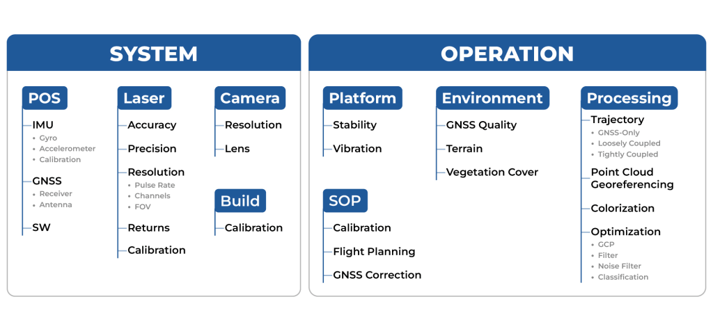
Figure 1. Factors that affect the accuracy of the point cloud.

Special attention is given to the high level of integration with other systems and filters, which significantly improves performance and data quality. In this article, you will learn why Inertial Labs’ INS is not just a solution but a true revolution in accuracy and reliability for your business.

Here are the sections that will be covered: “When every centimeter counts: the role of INS in LiDAR data accuracy,” Error Source: Why doesn’t the Kalman filter always solve the problem?”, “Why Inertial Labs’ INS outperforms the competition,” and “PPK: The key to LiDAR survey accuracy.” The conclusion will summarize the benefits of using Inertial Labs’ INS in LiDAR payloads.

Modern Applications Need Accurate LiDAR Mapping Data

Modern infrastructure and development projects require the creation of detailed and accurate terrain models, where minor errors can have significant consequences. In the construction industry, high-precision point clouds monitor progress, plan and control heavy equipment, and verify that finished projects meet design standards. When inspecting bridges, dams, or powerlines, high accuracy is often needed even in GNSS-denied environments (e.g., in urban areas or under dense vegetation). Digital twins are becoming more widely adopted in many industries. At the core of these solutions is a requirement for measuring precise position and orientation to ensure that each map element correctly aligns with the other, most often in a global coordinate system. All these applications need sensor-fusion mapping technologies with high positioning and orientation accuracy, which rely on a high-precision INS solution [2].

The development of INS technologies, such as those from Inertial Labs, not only helps solve these challenges but also sets new standards for accuracy and efficiency by making technologies that were once inaccessible to many industries within reach by driving cost-effective innovations. Inertial Labs INS integrated with RESEPI offers a unique combination of accuracy, functionality, and affordability [3].

Better INS Enables More Accurate LiDAR Mapping Data

For a navigation-based LiDAR mapping solution, the INS is a core system component. To create a georeferenced point cloud, the solution first needs to resolve the mission trajectory (its system positions and orientations at every timestamp), then project LiDAR points at each epoch of the trajectory using the LiDAR’s collected distance and scanning angle for each return. In this context, the performance of the INS becomes critical for the accuracy of the output point cloud because it offers the system the capability to measure global position and orientation, which is the reference from which the LiDAR points are projected. LiDAR can provide point clouds of very high density. Still, without accurate information about the system sources’ position and orientation in space, this data will be challenging to interpret (or unusable) because even minor errors in angular and linear measurements can lead to propagated errors over the entire project. For example, if the mistake along one of the x/y/z axes is 0.1 degrees, then at 50 meters the error in determining the coordinate will be off by about 17.5 cm. However, with an error of 0.01 degrees and the same distance, the mistake of determining the coordinate will be reduced to 1.75 cm. In short, precision and accuracy matter significantly when errors can compound.

In addition, the high accuracy of the INS in combination with LiDAR allows more efficient implementation of techniques such as LiDAR-based SLAM (Simultaneous Localization and Mapping), where one the most important contributors to the accuracy of the SLAM solution at each epoch is the motion model that can be derived from the data produced by the INS which is used to correct the map and trajectory estimation [10]. In such systems, an INS can provide data with a low error rate so that the system can better track changes in position and orientation. To accomplish this, systems typically use integrated solutions where data from INS and LiDAR are processed together through a Kalman filter. For such advanced systems, the accuracy of the INS data remains a basis for the correct and reliable operation of the SLAM algorithm without the risk of failure or instability introduced where LiDAR features or frame-to-frame motion render the algorithm unable to estimate its current state.

Thus, INS accuracy and stability become key to ensuring accuracy in LiDAR systems of various kinds, especially when integrated with other sensors and when using complex algorithms such as SLAM. Proper calibration and error minimization in INS sensors will maximize the use of LiDAR data, providing high-quality and accurate results in applications ranging from autonomous vehicles to geodetic surveys.

What Affects the Accuracy of Position and Orientation Determination?

At the “heart” of an inertial navigation system are Gyroscopes and Accelerometers [4]. Gyroscopes and Accelerometers form the basis of an Inertial Measurement Unit (IMU), providing data for calculating an object’s orientation, velocity, and position. Gyroscopes measure angular velocity around the three axes (X, Y, Z) using the effects of inertia, such as the Coriolis effect in MEMS gyroscopes, Figure 2 [5]. This data allows the current orientation of an object to be determined through the integration of angular velocities. However, gyroscopes have a bias and are also subject to systematic drift, which leads to an accumulation of angular error, as shown in Figure 3. Also, let’s not forget about random noise causing additional measurement errors. In addition, their sensitivity or errors can vary with temperature, which requires correction algorithms [6].

Figure 2. IMU designation.

Accelerometers, in turn, measure linear acceleration in three axes, capturing changes in object motion linearly. They can determine orientation from gravitational acceleration under static conditions and even calculate an object’s local position through the double integration of accelerations. However, accelerometers are also susceptible to zero drift. Random noise and vibrations exacerbate this problem, reducing the accuracy of measurements under dynamic conditions.

Figure 3. Gyroscope bias and drift.

To compensate for these errors, filters and algorithms, such as the Kalman filter, combine IMU data with external sources (e.g., GNSS or magnetometer), smoothing noise, and correcting for accumulated errors [6]. Many filters attempt to use the best of each available sensing component offering, using the other to correct for its faults.

However, even the most advanced algorithms cannot eliminate systematic drift or error, making sensor quality, zero drift minimization, and stability of sensor performance critical for high-precision IMU operation.

Why Can’t the  Kalman Filter Fully Compensate for Errors?

The Kalman filter is a powerful tool for processing sensor data and improving the accuracy of system state estimation, but its ability to compensate for IMU errors has limitations. The main problem is that the Kalman filter assumes a linear model of the system dynamics and the best knowledge of the statistical properties of the noise. In reality, many IMU errors, such as gyro and accelerometer drift, are nonlinear and time-varying, making it difficult to compensate for them entirely using a standard Kalman filter. In addition, the Kalman filter requires accurate noise models. Still, in the case of IMUs, noise often depends on multiple factors such as temperature, vibration, or electromagnetic interference, making it challenging to model and account for in the filter.

The following methods are commonly used to compensate for such errors:

• Long-term Calibration. Sensors are tested in a laboratory environment to determine the static zero offset. The calibration parameters are stored in the microcontroller. This approach is used in most commercial IMUs.
• Baseline Averaging. The average of the steady-state readings is determined and then subtracted from the current data.
• Thermal Compensation. Temperature-dependent offset models are created based on laboratory measurements. Linear approximation, polynomial approximation, or exponential models are often used.
• Temperature Sensors. Built-in temperature sensors record the current temperature, and the algorithm adjusts it based on the temperature model.

These are basic and commonly used methods that can be integrated into the Kalman filter, but in general, the filter itself cannot correct all the IMU errors, as shown in Figure 4.

Figure 4. The result of the Kalman filter.

The Kalman filter is described by two main equations: prediction equations and update equations. The covariance matrices and play a key role in these equations, determining how the filter accounts for system dynamics and measurement uncertainty.

Prediction Equations estimate the state and error covariance based on the system model (4):

                                                              (4)   

where  is the predicted state of the system,  is the state transition matrix (dynamic model);   is the control matrix,  is the control vector, is the expected error covariance, and is the process noise covariance matrix.

A larger indicates less trust in the model and more reliance on measurements. A smaller increases trust in the predicted dynamics.

Update Equations to correct the prediction using new measurements (5):

                                                                (5)

where  is the Kalman gain (weighting coefficients);  is the measurement vector; is the measurement matrix (links the state to the measurements), and is the measurement noise covariance matrix.

A larger  indicates less trust in the measurements. A smaller increases the influence of measurements on the final state.

To improve the performance of the Kalman filter, several key approaches can be applied:

• First, carefully tuning the process and measurement noise is essential. Noise parameters Q and R significantly affect the accuracy of the filter. Improperly chosen values can cause the filter to either trust the measurements too much (in the case of too low a value for R) or not account for them properly (if R is too large). Adaptive methods are often used for more accurate modeling to adjust these noises as the filter performs dynamically.
• Second, in the case of using a Kalman filter for nonlinear systems, it may be necessary to use an extended Kalman filter (EKF) that approximates the nonlinearities using linear approximations. This requires appropriately developing nonlinear models for states and measurements and the computation of their Jacobians. It is vital to ensure that these models accurately reflect the fundamental processes of the system so that the filter can update its estimates correctly.
• A third important point is the proper initialization of the initial conditions. If the initial values of the condition or covariance are chosen too far from the fundamental values, the filter may take a long time to converge or sometimes not converge. Using more accurate estimates of initial states or performing pre-filtering for correct initialization is recommended.
• Combined methods can also be used, such as a Kalman filter using multivariate data or combining the Kalman filter with other methods, such as particle filtering, to improve robustness and accuracy in the face of high noise or dynamic changes in the system. It is also worth considering implementing models to account for sensor drift, such as gyroscopes and accelerometers. This can significantly improve the long-term accuracy of the filter if drift is a significant factor in the system.

Thus, to improve the efficiency of the Kalman filter, it is essential not only to tune the filter parameters properly but also to deeply understand the dynamics of the system the filter is working with and to pay attention to possible improvements to the models and computational methods.

Using Multidimensional Data or What is Sensor Fusion

Using external data from different sensors (Sensor Fusion) can significantly improve the accuracy and robustness of the Kalman filter, especially in complex applications such as positioning and navigation systems [7]. Incorporating additional sensors into the filtering process can compensate for inefficiencies and errors that may arise due to noise or limitations of individual sensors.

The incorporation of data from external sensors such as GPS, magnetometers, or barometers can compensate for gyro drift and reduce the accumulation of errors in integrated measurements, especially in long-duration measurements. In addition, dynamic environmental data, such as data from a camera, can further improve positioning in complex or poorly controlled environments, such as urban canyons or enclosed spaces [8].

In addition, using external data also helps make the filter more resilient to abnormal situations or sensor malfunctions. For example, suppose one of the sensors fails or starts giving false data. In that case, the filter can automatically adapt and rely on other, more reliable sources of information, minimizing the effect of the malfunction. For example, this could be GNSS signal spoofing (spoofing) or jamming, so the algorithm will not use GNSS data but rely on odometer and/or barometer data [9].

Thus, external data can significantly improve the accuracy and robustness of the Kalman filter, providing more robust and adaptive solutions, especially under uncertainty or with limited internal measurements.

Why Inertial Labs INS Outperforms Competition

RESEPI utilizes a variation of the IMU Kernel-210 with high-accuracy gyroscopes and accelerometers. We compared its characteristics with commonly used competitor solutions and provided an understanding of where they sit when comparing prices. The comparison results are shown in Table 1. Let’s understand what these parameters mean and how they affect accuracy.

Table 1. Comparison of IMU Kernel-210 characteristics with competitors.

The declared datasheet values are often measured under ideal laboratory conditions. To this end, manufacturers carry out special calibration procedures to determine the errors of their IMUs. The values provided in Table 1 are residual errors after thermal calibration. The sensors are calibrated over a wide temperature range—in this case, from –40 to 85 degrees Celsius—to ensure functionality in real-world conditions.

Gyro Bias repeatability. The “bias” of a gyroscope is the angular velocity value that the gyroscope indicates when it is stationary. Ideally, these values should be zero, but in real devices, they may have a nonzero value at rest due to sensor peculiarities.

“Repeatability” shows how consistently this offset (within the specified temperature range) occurs every time the gyroscope is turned on and off. Good repeatability means the bias will be approximately the same at each startup; poor repeatability implies that the bias may vary noticeably from one startup to the next. As can be seen, the KERNEL-210 has the lowest value, so temperature changes will affect its accuracy much less compared to competitors, whose bias is over eight times larger.

Gyro bias in-run stability. “In-run stability” indicates how much the gyroscope’s bias changes during operation. Even if the bias is well-calibrated at startup, it may “drift” or change slowly over time. High stability means that the bias remains almost constant over long periods of operation.

Gyro Scale Factor error.  “Scale Factor error” is the deviation of the scale factor from its ideal value. This means the gyroscope may output slightly different values for the same actual angular velocity due to the scale factor error.

ARW. “Angular Random Walk” is a characteristic that describes the random noise in the gyroscope’s output signal. It measures how the integrated angle drifts randomly due to this noise. Even without drift and zero scale factor error, ARW will introduce random and unpredictable errors in the orientation estimation, accumulating over time following a random walk process (roughly proportional to the square root of time).

Since we have clarified the differences and the importance of these parameters, let’s consider their impact on orientation accuracy.

For assessing the accuracy of such extensive and complex systems as an INS, it is common to simulate the system’s performance under various conditions (stationary base, rocking, accelerated motion, etc.). However, for a simple error estimation, one can use the simplified formulas of the gyroscope signal model [10].

For gyroscopes, the impact of drift on the accuracy of angle measurements with a stationary base can be estimated using equation (1). In this case, we assume that the drift is constant.

                                                                          (1)

where is the gyroscope drift, and is the operating time without external correction.

The impact of noise is expressed by equation (2):

                                                               (2)

where  is the gyroscope noise (or Angular Random Walk) .

The scale factor error is expressed by equation (3):

                                                                  (3)

where is the scale factor error ,  is the angular speed

To determine which parameters have the most significant influence, we substitute the values from Table 1 for the KERNEL-210 and calculate the errors for each component. In doing so, we set the time t = 60 sec and assume   is operating within its’ worst-case scenario, i.e., as the sum of both biases: Gyro Bias repeatability and Gyro bias in-run stability. We will also assume that the angular velocity = 3 deg/s. The result of the angular measurement accuracy calculation is shown in Table 2.

Table 2. Angle measurement accuracy calculation result.

As can be seen from the results, the most significant sources of error are bias and scale factor error.

By integrating the acceleration (accelerometer signal) twice, we obtain the displacement value, or, in other words, the change in position. The effect of the zero offset can be estimated using the formula (4) [11]:

                                                        (4)

where  is the accelerometer bias  .

The effect of the scale factor shift is estimated using the formula (5):

                                                                     (5)

where  is the scale factor error , and is the distance traveled .

The error caused by VRW noise is expressed by the following formula (6):

                                                                    (6)

where  is accelerometer noise (or Velocity Random Walk)  .

As with gyroscopes, we also substitute the values from Table 1 for the KERNEL-210 and calculate the errors for each component. In doing so, we set the time t = 60 sec and assume is operating within its’ worst-case scenario, i.e., as the sum of both biases: Accel Bias repeatability and Accel bias in-run stability. We will also assume that the distance = 1000 m. The result of the coordinate accuracy calculation is shown in Table 3.

Table 3. Angle measurement accuracy calculation result.

As can be seen from the results, the most significant sources of error are bias and scale factor error.

To demonstrate the superiority of the KERNEL-210, we calculated the errors under the same conditions using the specifications of competing solutions from Table 1. The result is shown in Table 4.

Table 4. Result of IMU KERNEL-210 comparison.

The outcome demonstrates the advantages of the KERNEL-210 IMU compared to its competitors. Despite being somewhat inferior in noise characteristics compared to the competitive landscape, some performance characteristics come at a significant cost difference. The gyroscopes in KERNEL-210 achieve high accuracy due to superior performance in parameters that are far more important than noise. As a result, when integrated into systems like RESEPI, users can expect to see point clouds with reliable accuracy when surveying applications.

The Kernel-210 IMU is designed to operate in harsh environmental conditions and, as mentioned, has a high reliability rating. MTBF (GM @+65degC, operational) is 100000 hours. Long service life and stable operation reduce maintenance and replacement costs. No one wants to interrupt work and face losses due to the need for IMU maintenance or calibration.

Additionally, our IMU provides a high data update rate of 2000 Hz. A higher frequency allows for faster movements to be tracked.

We conducted real-world tests and scanned a section of territory with the RESEPI XT32 at a 100 km/h speed, as shown in Figure 5. The flight altitude was about 50 m, the recommended AGL for this model, and was used on a manned aircraft.

Figure 5. RESEPI velocity chart during operation.

The point cloud obtained in this way is shown in Figures 6 and 7. As you can see, the relative accuracy is just over 4 cm. This explanation aims to showcase the benefit of higher update rates and their impact on data quality. Although fully capable, as seen in other papers, for use on VTOL aircraft and multi-rotor UAVs, RESEPI is not limited to these platforms and can be used on larger vehicles, even manned aircraft.

Figure 6. General view of the point cloud.

Figure 7. Relative accuracy of about 4 cm.

Looking at all things considered when comparing IMU specifications and results, the KERNEL-210 is not the absolute leader from what was shown in terms of drift parameters on paper. Still, for performance at the right price, the KERNEL-210 leads in its class. In real-world LiDAR Payload operation, the difference in accuracy becomes almost imperceptible, while you get significant savings in cost and size. No, we are not saying that error characteristics are unimportant. Still, for most LiDAR payload applications, such as surveys, mapping, and geodetic measurements, the key factor is the overall system efficiency, not just the parameters of a single sensor element. Our IMU, combined with a GNSS receiver, adaptive algorithms, and a high-precision LiDAR, provides an optimal balance of accuracy, cost, and practicality. However, as we will discover, data post-processing also plays a significant role.

The following section will examine the importance of post-processing raw data.

PPK: Another Key to LiDAR Data Accuracy

RTK (Real-Time Kinematics) provides highly accurate real-time coordinate correction, but this technology has risks. One major factor is the dependence on a stable connection to a base station or RTK network, which becomes problematic in remote areas, mountainous terrain, dense forests, or urban canyons. Loss of signal, even briefly, can result in a dramatic drop in accuracy or a complete shutdown. In addition, RTK quality depends on having a reliable GNSS signal, which can be disrupted by weather or interference.

Real-time technologies such as RTK are not always up for the challenge when operations depend on millimeter accuracy. On the other hand, PPK (Post-Processed Kinematics) provides the flexibility and reliability that LiDAR data processing requires and that typical surveyors need. PPK lets you focus on collecting data, knowing its accuracy will be restored during post-processing.

NovAtel’s Inertial Explorer by Waypoint is a powerful GNSS and inertial data post-processing tool that significantly simplifies the integration of PPK into LiDAR workflows, Figure 8. This software package combines sophisticated GNSS+IMU data processing algorithms to minimize positioning errors and achieve exceptional accuracy [12].

Integrating Inertial Explorer into the PCMasterPro LiDAR data processing software makes the complete workflow for users efficient and convenient [13]. The software automatically synchronizes data from base stations, provides GNSS information correction, and uses IMU data to improve accuracy.

Figure 8. Post-processing software.

The use of the KERNEL-210 IMU in combination with NovAtel’s Inertial Explorer optimized in PCMasterPro significantly improves the quality of acquired data, ensuring the highest accuracy in challenging conditions.

Let’s look at the position and orientation accuracy graphs of the post-processed data from RESEPI, which are shown in Figures 9 and 10. They show the accuracy of positioning and orientation over the entire data acquisition. The heading accuracy graph does not exceed 0.6 arcmin, approximately 0.01 deg. The roll and pitch accuracy does not exceed 0.3 arcmin = 0.005 deg. We did not consider the takeoff and landing sections, where the error is about 1.7 arcmin, since the data obtained at these moments usually show the runway. How often do you see results from using a product that exceeds the values advertised on a datasheet?

Figure 9. Attitude Accuracy Plot.

On the positioning accuracy graph, all three components (East, North, and Height) are within 1 cm.

Figure 10. Position Accuracy Plot.

Post-processing increased the point cloud’s final accuracy, making it suitable for actual use in surveying applications.

That is why considering such complex systems as LiDAR Payload, focusing only on the IMU, is wrong. Here, a comprehensive approach plays a role, which includes not only hardware solutions but also software.

Conclusion

The high-performance INS integrated into Inertial Labs’ RESEPI solution is an advanced Inertial Navigation System for applications requiring high accuracy and robustness, with powerful sensor technology, minimal requirements for regular calibration, and support for flexible integrations with other navigation technologies. This INS enables RESEPI systems to achieve the best possible data for LiDAR survey or mapping professionals, offering the tools to efficiently and reliably complete challenging projects across various use cases.

Inertial Labs is committed to providing our global customers with high-quality solutions and excellent values at affordable costs. Attitude is Everything!

References

[1] “LIDAR Market Size to Hit USD 13.74 Billion by 2033.” Www.precedenceresearch.com, www.precedenceresearch.com/LiDAR-market.

[2] Mendez, Maria. “Why Use a Survey-Grade INS on a UAV?” Inertial Labs, 25 Nov. 2024, inertiallabs.com/why-use-a-survey-grade-ins-on-a-uav/.

[3] “RESEPI – LiDAR Payload & SLAM Solutions.” RESEPI, 12 July 2024, LiDARpayload.com/.

[4] Aboelmagd Noureldin. Fundamentals of Inertial Navigation, Satellite-Based Positioning and Their Integration. Heidelberg, Springer, 2013.

[5] “MEMS.” Wikipedia, 26 Apr. 2023, en.wikipedia.org/wiki/MEMS.

[6] BOSE, AMITAVA, et al. FUNDAMENTALS of NAVIGATION and INERTIAL SENSORS. PHI Learning Pvt. Ltd., 1 Jan. 2014

[7] Mendez, Maria. “Integrating INS with Aiding Data Technologies – the INS Ecosystem RoadMap.” Inertial Labs, 29 Apr. 2024, inertiallabs.com/integrating-ins-with-aiding-data-technologies-the-ins-ecosystem-roadmap/. Accessed 25 Sept. 2024.

[8] Mendez, Maria. “VIO Revolution in Navigation and Positioning.” Inertial Labs, 4 Dec. 2024, inertiallabs.com/vio-revolution-in-navigation-and-positioning/. Accessed 15 Jan. 2025.

[9] Oleh Omelianenko. “Aiding Data Examples and Use Cases for the Inertial Labs INS.” Inertial Labs, 12 Feb. 2024, inertiallabs.com/aiding-data-examples-and-use-cases-for-the-inertial-labs-ins/. Accessed 15 Jan. 2025.

[10] Derya Unsal, and Kerim Demirbas. “Estimation of Deterministic and Stochastic IMU Error Parameters.” OpenMETU (Middle East Technical University), 1 Apr. 2012, https://doi.org/10.1109/plans.2012.6236828. Accessed 22 Mar. 2024.

[11] Borodacz, Krystian, et al. “Review and Selection of Commercially Available IMU for a Short Time Inertial Navigation.” Aircraft Engineering and Aerospace Technology, vol. 94, no. 1, 26 July 2021, pp. 45–59, https://doi.org/10.1108/aeat-12-2020-0308. Accessed 10 Mar. 2025.

[12] Waypoint Post-Processing Software. 2023, novatel.com/products/waypoint-post-processing-software.

[13] Mendez, Maria. “Understanding the Need for Post-Processing in GPS Data.” Inertial Labs, 8 Jan. 2025, inertiallabs.com/understanding-the-need-for-post-processing-in-gps-data/. Accessed 15 Jan. 2025.

The post Deep Dive into RESEPI Accurate Data appeared first on RESEPI.

This article discusses the key factors to consider when selecting an Inertial Navigation System (INS) for mobile mapping. Five key aspects are highlighted: accuracy level, cost, compatibility with other sensors, and system functionality. The calibration issue is also touched upon as an essential component affecting accuracy. It is emphasized that balancing the required accuracy and cost is crucial, avoiding overpaying for unnecessary features or high accuracy that is not critical to the application.

The sections will cover Introduction to INS, INS selection criteria for mobile mapping, and Mobile mapping INS from Inertial Labs. The conclusion will summarize the benefits of using Inertial Labs’ solutions for mobile mapping.

Section 1. Introduction to INS

An inertial navigation system (INS) is a device that uses gyroscopes and accelerometers (the main components of an inertial measurement unit – IMU), and sometimes magnetometers, to calculate an object’s orientation angles, position, and velocity without relying on external data sources [1].

The operating principle of an INS involves accelerometers measuring the acceleration (“Accel”) of the object along different axes (typically three mutually perpendicular axes – X, Y, and Z). In contrast, gyroscopes measure the angular velocity (“Gyro”) of the object’s rotation relative to these axes, as shown in Figure 1. This enables the tracking of changes in the object’s spatial orientation. [2].

Figure 1. Location of gyroscopes and accelerometers in the IMU.

Initially, the accelerometers measure acceleration, which is then integrated over time to find the object’s velocity. This velocity is further integrated to compute the object’s current position in space. Gyroscope signals are also integrated to determine the orientation angles, including pitch, roll, and yaw.

Because inertial sensors can experience errors like gyro drift and accelerometer noise, filters such as the Kalman filter are applied to reduce these errors and correct drifts [3]. The INS is often combined with a GNSS system to address these inaccuracies and correct accumulated errors. However, when the GNSS signal is lost for an extended period, the errors increase, which becomes particularly significant over long distances. Therefore, while the INS is suitable for autonomous navigation, additional correction techniques are necessary to maintain accuracy[4].

Now that we have reviewed the basic principles of INS operation let us examine the criteria for selecting INS for mobile mapping. Those readers who want to understand the work of INS better can find more information at the links [5, 6].

Section 2. INS selection criteria for mobile mapping

Data accuracy and stability

This is the most important criterion that will determine the accuracy of the user’s maps. Since additional sensors such as LiDAR or cameras are often used for mapping, the slightest inaccuracy in determining the vehicle’s angles and the data collection system will lead to significant errors in mapping.

As was said in the previous section, one of the features of INS operation is the accumulation of errors in the absence of external correction sources, such as GNSS. Unique methods and algorithms, such as Tightly Coupled, improve the system’s accuracy and reliability.

Tightly Coupled is a variant of the INS architecture that uses a standard Kalman filter to estimate INS errors, Figure 2. “The difference between the pseudo-range and pseudo-range rate measurements from the GPS and corresponding values predicted by the INS are fed to the KF to estimate the errors in the INS. The output from the INS is then corrected for these errors to obtain the integrated navigation solution. It is possible to use either pseudo-range or pseudo-range rate measurements, but often both are used because they are complementary.” [6].

Figure 2. Tightly Coupled architecture.

“The tightly coupled integration eliminates the problem of correlated measurements arising from cascaded Kalman filtering in the loosely coupled approach. Furthermore, this integration provides a GPS update even if fewer than four satellites are visible. This is useful because a typical real-life trajectory includes urban environments, thick forest canopies, and steep hills where the number of visible satellites can drop to fewer than four.” [6].

Compatibility with other sensors

Another integration approach is Sensor Fusion [7]. Sensor Fusion involves using additional sensors, which are the information used to correct INS in the absence of GNSS. Such sensors include encoders, odometers, barometers, Doppler Velocity Log (DVL), etc. [8].

Since mobile mapping involves using a car (although it is not the only option), we recommend paying attention to INS support Sensor Fusion, particularly odometry, which is used to determine distance based on the rotation of the vehicle’s wheels. Also, a helpful addition would be using DVL to determine speed. Sensor Fusion is an excellent addition to your INS correction without a GNSS signal, especially if you plan to work outside.

Operating conditions and reliability

Mobile mapping can take place in a variety of locations and conditions. It can be dry, wet, cold, or hot climates. When choosing a system, it is essential to be sure that no conditions, even the most difficult ones, will affect its operation.

Therefore, when choosing an INS, you should consider its protection level. According to IEC 60529 standards, the protection level code is “IPXX” [9]. It is essential that the INS is protected from moisture and dust, as well as from impacts. It is equally important to know the average service life of the system.

Cost and long-term benefit

When choosing an INS, accuracy is essential, but so is price. It is only sometimes worth paying more for higher accuracy, as some INS may offer data with more accuracy than required. Generally, the higher the accuracy, the higher the cost, so you may pay more than you need. A system that costs twice as much will be less accurate. Therefore, it is recommended that you analyze the entire range and determine what accuracy and features you need. This will allow you to save money by excluding features and functions you do not need.

Recalibration required during service life

The IMU has features such as a transfer coefficient (scale factor), zero offset, cross-links, and other parameters. In addition, when installing sensitive elements in the IMU, due to instrumental manufacturing errors, there are mismatches between the sensitivity axes of the elements and the base axes of the unit. To ensure high accuracy of the INS, it is necessary to have highly accurate information from the measuring devices, which can only be ensured by considering the specified features of each accelerometer and gyroscope. Calibration consists of determining the parameters of the measuring devices to compensate for instrumental errors in the navigation mode. The accuracy of the output orientation parameters depends on the quality of the INS calibration.

Calibrations are usually performed on special high-precision stands that provide the operating temperature range according to the declared characteristics of the system. This is important because not only instrumental errors affect accuracy but also temperature.

Many manufacturers provide information about the need for recalibrations, which is often a paid service; at the same time, there is a high probability that you will have to send the INS back to the manufacturer, which will lead to downtime, thereby depriving you of profit. In this regard, when choosing an INS, you should carefully study these nuances to reduce the risks of losing time and money in the future.

Now that we’ve covered five essential criteria let’s look at what Inertial Labs offers and why it’s the best choice for mobile mapping.

Section 3. Mobile mapping INS from Inertial Labs

The Inertial Labs Single and Dual Antenna GPS-Aided Inertial Navigation System – INS is a new generation of fully integrated, combined GPS, GLONASS, GALILEO, QZSS, BEIDOU, and L-Band navigation and high-performance strapdown system that determines position, velocity and absolute orientation (Heading, Pitch, and Roll) for any device on which it is mounted. Horizontal and Vertical Position, Velocity, and Orientation are determined with high accuracy for both motionless and dynamic applications.

The professional model of INS, the INS-P, utilizes an embedded, high-precision, gyro-compensated magnetic compass, which allows the navigation system to measure and output high-precision Heading without GNSS signal even in extreme environmental conditions (temperature, vibration, interference from external magnetic field), Figure 3 [10].

Figure 3. The INS-P.

Systems have Tightly Coupled support and Sensor Fusion to provide the user with reliable and accurate data in conditions of GNSS signal loss, Figure 4. All systems have an IP67 protection class, guaranteeing uninterrupted operation even in the harshest conditions. The average service life of the systems is more than 10 years, and the user does not have to worry about recalibrations since the factory calibrations are enough for the entire operating life.

Figure 4. Technical characteristics and functionality of INS from Inertial Labs.

The reliability of the systems is confirmed by military standards MIL-STD-810 and RTCA-DO-160E. Therefore, we guarantee stability and failure-free operation over a wide temperature range (-40 to +75 C).

We offer a wide range of systems and the ability to customize them to your needs, so you don’t pay for what you don’t need.

The Inertial Labs team of skilled engineers provides expertise to help users select and configure from the available models. Our support team helps set up units for all application bases to satisfy GNSS-enabled and GNSS-denied environments.

Conclusion

In conclusion, choosing an inertial navigation system (INS) for mobile mapping requires a balanced approach that balances accuracy, cost, functionality, and system compatibility. Understanding the specific project requirements and carefully analyzing available solutions will help you avoid unnecessary costs and select the most appropriate device to provide optimal performance without overpaying for unnecessary features.

Additionally, the capabilities of inertial systems from Inertial Labs are reviewed. With extensive integration capabilities, support for external sensors, accuracy, and reliability, these systems are an excellent choice for mobile mapping.

Among the many developers, Inertial Labs stands out for offering customizable solutions that meet the unique needs of different applications. Their systems are designed to be easily integrated with a wide range of external sensors, allowing for flexibility that improves system performance and simplifies user integration. This approach not only simplifies development but also significantly reduces the associated costs.

References

[1] Wikipedia Contributors. “Inertial Navigation System.” Wikipedia, Wikimedia Foundation, 21 May 2019, en.wikipedia.org/wiki/Inertial_navigation_system.

[2] Aboelmagd Noureldin. Fundamentals of Inertial Navigation, Satellite-Based Positioning and Their Integration. Heidelberg, Springer, 2013.

[3] Wikipedia Contributors. “Kalman Filter.” Wikipedia, Wikimedia Foundation, 27 Mar. 2019, en.wikipedia.org/wiki/Kalman_filter.

[4] Mendez, Maria. “Integrating INS with Aiding Data Technologies – the INS Ecosystem RoadMap.” Inertial Labs, 29 Apr. 2024, inertiallabs.com/integrating-ins-with-aiding-data-technologies-the-ins-ecosystem-roadmap/. Accessed 25 Sept. 2024.

[5] Wikipedia Contributors. “Inertial Navigation System.” Wikipedia, Wikimedia Foundation, 21 May 2019, en.wikipedia.org/wiki/Inertial_navigation_system.

[6] Aboelmagd Noureldin. Fundamentals of Inertial Navigation, Satellite-Based Positioning and Their Integration. Heidelberg, Springer, 2013.

[7] Wikipedia Contributors. “Sensor Fusion.” Wikipedia, Wikimedia Foundation, 30 June 2019, en.wikipedia.org/wiki/Sensor_fusion.

[8] Mendez, Maria. “Integrating INS with Aiding Data Technologies – the INS Ecosystem RoadMap.” Inertial Labs, 29 Apr. 2024, inertiallabs.com/integrating-ins-with-aiding-data-technologies-the-ins-ecosystem-roadmap/. Accessed 25 Sept. 2024.

[9] “IEC 60529:1989+AMD1:1999+AMD2:2013 CSV.” Webstore.iec.ch, 2015, webstore.iec.ch/en/publication/2452.

[10] “INS – GPS-Aided Inertial Navigation Systems.” Inertial Labs, 13 Aug. 2024, inertiallabs.com/products/ins-inertial-navigation-systems/. Accessed 25 Sept. 2024.

The post Five considerations when selecting an INS for mobile mapping appeared first on RESEPI.

With a lightweight design for easy transport and deployment, the RESEPI Ultra LITE is compatible with numerous platforms, including Freefly, WISPR, DJI, Sony, and mobile setups. This seamless integration is achieved through Inertial Labs’ proprietary SnapFit adapters, which ensure rapid and secure mounting and dismounting. Cost-effective and entering the market at an MSRP pricing of $18,800 without compromising quality, the RESEPI Ultra LITE delivers on affordability, providing high value for professionals needing precision without exceeding budget constraints. Engineered for high accuracy and precision, the system underwent meticulous testing to refine timestamping and calibration methods, empowering users to capture data confidently.

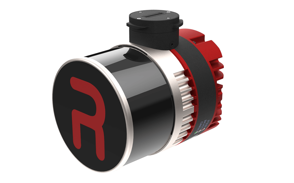
Inertial Labs CEO Jamie Marraccini commented, “Inertial Labs has always aimed to push the boundaries of survey technology, and the RESEPI Ultra LITE exemplifies our commitment to delivering high-performance tools that don’t compromise on quality or value. Combining the lightest and most adaptable design with best-in-class precision empowers surveyors and 3D mapping professionals to capture data faster, easier, and more confidently.”

The RESEPI Ultra LITE’s compact configuration includes a 5MP colorization camera, making it an ideal solution for SUAS platforms with volume constraints requiring LiDAR and camera capabilities. It shines in aerial and ground-based applications, such as utility mapping (power lines), construction volumetrics, precision agriculture, forestry, site surveying, and mining. Built to enhance efficiency and accuracy, the RESEPI Ultra LITE is an affordable and robust solution providing high investment returns for 3D mapping and surveying professionals focused on cost efficiency and data quality.

About Inertial Labs

With over 20 years of industry experience, Inertial Labs is a leading designer, integrator, and manufacturer of cutting-edge Inertial Measurement Units (IMUs), GPS-aided inertial Navigation Systems (INSs), and Attitude and heading Reference Systems (AHRSs). Our team leverages highly accurate and temperature-calibrated MEMS gyroscopes and accelerometers to provide high-performing inertial solutions across many applications.

As experts in sensor fusion, Inertial Labs designs and develops quality products at the best price-performance ratio. Our team provides solutions capable of utilizing data from an array of sources, including air data computers (ADCs), ToF Mesh-Based Software-Defined Radios (SDRs), Visual Odometry, Air Speed Sensors, Odometers, Encoders, and Standalone Magnetic Compasses (SAMCs).

Inertial Labs is a lead developer of exciting technologies. Solutions include Inertial Sensing, Assured Position Navigation and Timing (APNT), GNSS Tracking, LiDAR Scanning, Alternative Navigation (ALTNAV), Visual Navigation, and Programmable Navigation Solutions.

For media inquiries, please contact:

Marketing Department

Email: [email protected]

Phone: +1 (703) 880-4222

Website: www.inertiallabs.com

The post Inertial Labs Unveils the Lightest Complete LiDAR and Camera Payload: The RESEPI Ultra LITE appeared first on RESEPI.