In particular, I showed that $A$ is a monotone operator and that the $f$ -resolvent $(\nabla f + \lambda A)^{-1} \circ \nabla f$ is Bregman firmly nonexpansive with respect to the Bregman divergence $D_f$. In other words, this ensures that this generalized PPA will converge to a fixed point, if there exists any.

In this blog post, we propose to generalize the gradient flow ordinary differential equation (ODE) by letting $\lambda \rightarrow 0$ in our generalized PPA (for a great introduction to gradient flow, see Bach’s blog post).

Definition: Let $F(x,q) = q^\intercal \ell(x)$. We define the barygradient flow ODE as \(\dot \zeta(t) = - \begin{pmatrix} I_m & 0 \\ 0 & -I_S \end{pmatrix} \nabla F( (\nabla f)^{-1}( \zeta(t) -\log(\sum_s e^{\xi_s(t)-1}) \begin{pmatrix} 0_m \\ 1_S \end{pmatrix} ) ) + \gamma(t) \begin{pmatrix} 0_m \\ 1_S \end{pmatrix} ,\) where $\zeta = (x,\xi) : \mathbb{R}_+ \rightarrow \mathbb{R}^m \times \mathbb{R}^S$ and \(\gamma(t) = \frac{\sum_s [ \dot \xi_s(t) - \ell_s(x(t)) ] e^{\xi_s(t)-1}}{\sum_s e^{\xi_s(t)-1}} = q(t)^\intercal [ \dot \xi(t) - \ell(x(t)) ]\) with $q(t)=(\nabla h)^{-1}(\xi(t)-\log(\sum_s e^{\xi_s(t)-1}) 1_S)$.

We point out that \(\begin{pmatrix} I_m & 0 \\ 0 & -I_S \end{pmatrix} \nabla F( (\nabla f)^{-1}( \zeta(t) -\log(\sum_s e^{\xi_s(t)-1}) \begin{pmatrix} 0_m \\ 1_S \end{pmatrix}) ) = A(x(t), q(t)) .\)

Monotonicity analysis

Contrary to classic gradient flow, the function $F(x(t),q(t))$ is not necessarily nonincreasing along the flow. Indeed, \(\frac{d}{dt}F( (\nabla f)^{-1}( \zeta(t) -\log(\sum_s e^{\xi_s(t)-1}) \begin{pmatrix} 0_m \\ 1_S \end{pmatrix} ) ) = \frac{d}{dt}[(\nabla h)^{-1}(\xi(t)-\log(\sum_s e^{\xi_s(t)-1}) 1_S)]^\intercal \ell(x(t)) + q(t)^\intercal \frac{d}{dt} \ell(x(t)) ,\) where \(\frac{d}{dt}[(\nabla h)^{-1}(\xi(t)-\log(\sum_s e^{\xi_s(t)-1}) 1_S)] = [\nabla^2 h(q(t))]^{-1} \dot \xi(t) - \frac{\sum_s \dot \xi_s(t) e^{\xi_s(t)-1}}{\sum_s e^{\xi_s(t)-1}} q(t)\) and $\frac{d}{dt} \ell(x(t)) = J_\ell(x(t)) \dot x(t)$.

Hence, \(\frac{d}{dt}F(x(t),q(t)) = \underbrace{ \ell(x(t))^\intercal [\nabla^2 h(q(t))]^{-1} \ell(x(t)) - F(x(t),q(t))^2 }_{\text{Var}_{\tau \sim q(t)}(\ell_\tau(x(t)))} - ||J_\ell(x(t))^\intercal q(t)||^2 ,\) which is not necessarily nonpositive.

Entropy analysis

Denote $\chi(t) = h(q(t))$. Then, \(\frac{d}{dt} \chi(t) = \dot q(t)^\intercal \nabla h(q(t)) = \{ [\nabla^2 h(q(t))]^{-1} \dot \xi(t) - [q(t)^\intercal \dot \xi(t)] q(t) \}^\intercal \{\xi(t)-\log(\sum_s e^{\xi_s(t)-1}) 1_S\} \\ = \xi(t)^\intercal \underbrace{[ \text{Diag}(q(t))-q(t)q(t)^\intercal ]}_{\text{Cov}(q(t))} \ell(x(t)),\) where $\text{Cov}(q(t))$ denotes the covariance matrix¹ of the categorical distribution $q(t)$.

Remark: The barygradient flow can be equivalently rewritten as the following natural gradient flow: \(\dot \zeta(t) = - \begin{pmatrix} I_m & 0 \\ 0 & -\text{Cov}(q(t))^\dagger \end{pmatrix} \nabla \tilde F( \zeta(t) ) + [ \gamma(t) + \frac{1_S^\intercal \ell(x(t))}{S} ] \begin{pmatrix} 0_m \\ 1_S \end{pmatrix} ,\) where $\dagger$ denotes the Moore–Penrose pseudoinverse and \(\tilde F(x,\xi) = (\nabla h)^{-1}(\xi - \log(\sum_s e^{\xi_s-1}) 1_S)^\intercal \ell(x).\)

Definition: A function $F:\mathbb{R}^d \rightarrow \mathbb{R}$ is said cross-convex if there exists $S\ge 1$ log-concave functions $p_1,\dots,p_S$ such that \(\forall x\in \mathbb{R}^d , \ F(x) = -\log\left( \sum_{s=1}^S p_s(x) \right) .\)

If $S=1$, then a cross-convex function is simply convex. In the general case $S\ge 1$, we argue that this family of functions is still a natural one to consider as it includes the negative log-likelihood of the Gaussian mixture model.

Let us first recall that a differentiable function $f:\mathbb{R}^d \rightarrow \mathbb{R}$ is convex if it dominates all its tangent hyperplanes: \(\forall a, \forall x, f(x) \ge f(a) + \nabla f(a)^\top (x-a).\)

$\bullet$ Summation/Affine Closure: A very important characteristic of the family of convex functions is that it is closed under (i) summation and (ii) affine reparametrization. Formally, (i) if $f_1,f_2$ are two convex functions, then $f_1+f_2$ is also convex ; and (ii) if $f$ is convex, then $z \mapsto f(Az+b)$ is also convex. These two closure properties are very important in machine learning where the objective function is typically equal to a sum over the dataset with affine neuronal transformations of the input data. A first challenge when trying to generalize convexity for ML applications is to pick a family of functions satisfying such closedness under summation and affine reparametrization. For instance, while the notion of quasi-convexity is often cited as a natural extension of standard convexity, unfortunately it is not closed under summation since the sum of two quasi-convex functions is not necessarily quasi-convex.

Proposition: Let $F = -\log\left( \sum_{s=1}^S p_s \right)$ and $\tilde F = -\log\left( \sum_{s=1}^{\tilde S} \tilde p_s \right)$ be two cross-convex functions with $S,\tilde S \ge 1$ and $p_s,\tilde p_s : \mathbb{R}^d \rightarrow (0,+\infty)$ log-concave functions. Then, the sum $F+\tilde F$ is also cross-convex. Indeed, \(F+\tilde F = -\log\left( \sum_{s=1}^S \sum_{s'=1}^{\tilde S} p_s \tilde p_{s'} \right) ,\) where the product of two log-concave functions $p_s \tilde p_{s’}$ is also log-concave.

Moreover, the class of cross-convex functions is also closed under affine reparametrization (follows from the closedness of log-concave functions).

$\bullet$ Generalized convexity inequality: Note that the right-hand side in the convexity inequality, namely “$f(a) + \nabla f(a)^\top (x-a)$”, represents the tangent hyperplane of $f$ at the point $a$. In particular, this lower bound is a critical ingredient in the analysis of gradient descent (see e.g. Bach’s LTFP book).

Key Remark: For any element $\mu \in [0,1]^S$ of the probability simplex (i.e., $\lVert \mu \rVert_1=1$), the KL-regularized log-loss \(\ell_\mu(x) = -\log( p_1(x)+\dots+p_S(x) ) + D_{\text{KL}}\left( \mu \Bigg\| \left[ \frac{p_s(x)}{ \sum_{s'} p_{s'}(x) } \right]_{s} \right)\) is convex.

In the following, we explain step-by-step how to obtain a similar lower bound in the cross convex case. For simplicity, we focus on the very specific case $S=2, d=2$ and $p_1(x,y)=p_2(y,x)=p(x)$ for some log-concave function $p: \mathbb{R} \rightarrow (0,+\infty)$, which already unveils phenomena unseen in the convex scenario. We refer the reader to Lemma 1 in “Beyond Log-Concavity: Theory and Algorithm for Sum-Log-Concave Optimization”¹ for the more general statement.

Steps

• Given log-concave function $p$
• Compute cross-convex function $F(x,y)=-\log(p(x)+p(y))$
• Tangent lower bound $\mathcal{T}_{a,b}(x, y) \le F(x,y)$ at point $(a,b)$: \(\mathcal{T}_{a,b}(x, y) = F(a,b) + \nabla F(a,b)^\top \begin{pmatrix} x-a \\ y-b \end{pmatrix} - D_{\text{KL}}\left( \begin{pmatrix} \frac{p(a)}{p(a)+p(b)} \\ \frac{p(b)}{p(a)+p(b)} \end{pmatrix} \, \Bigg \| \, \begin{pmatrix} \frac{p(x)}{p(x)+p(y)} \\ \frac{p(y)}{p(x)+p(y)} \end{pmatrix} \right)\)
• Note: Actually, the negative sign in front of the KL is bad news for the analysis of gradient descent…check out my paper to see how to solve that issue, by considering a reweighted version of the gradient

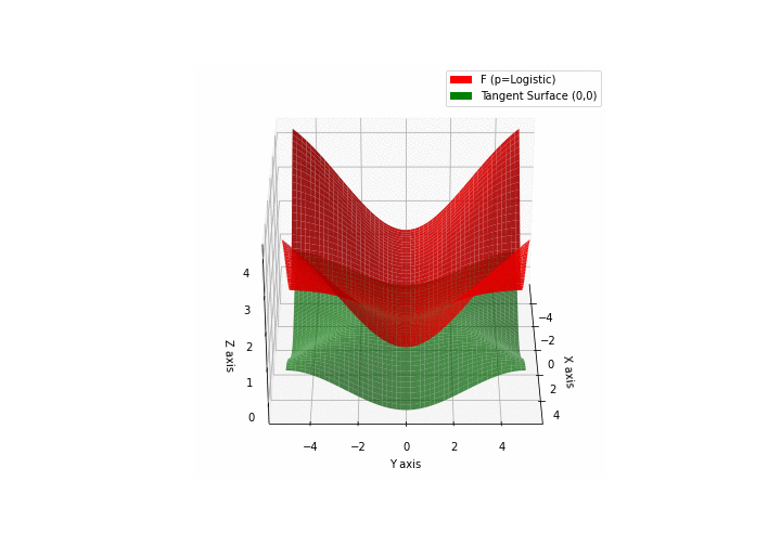
$\bullet$ \(\mathfrak{B}\)estiary: Collection of illustrations of cross-convex functions (in red) with their tangent surface (in green): https://github.com/mastane/TheXCB. The green tangent surface represents the lower bound $\mathcal{T}_{0,0}$ in the generalized convexity inequality.

• \(\mathcal{G}\)aussian mixture

• \(\mathcal{L}\)ogistic mixture

• \(\mathcal{H}\)yperbolic \(\mathcal{S}\)ecant mixture

• \(\mathcal{G}\)umbel mixture