LLMFunctionObjects

This blog post proclaims and describes the Python package “LLMFunctionObjects” that provides functions and function objects to access, interact, and utilize Large Language Models (LLMs), like OpenAI, [OAI1], and PaLM, [ZG1].

The structure and implementation of the Python package closely follows the design and implementation of the Raku package “LLM::Functions”, [AAp1], supported by “Text::SubParsers”, [AAp4].

(Here is a link to the corresponding notebook.)


Installation

Install from GitHub

pip install -e git+https://github.com/antononcube/Python-packages.git#egg=LLMFunctionObjects-antononcube\&subdirectory=LLMFunctionObjects

From PyPi

pip install LLMFunctionObjects


Design

“Out of the box” “LLMFunctionObjects” uses “openai”, [OAIp1], and “google-generativeai”, [GAIp1]. Other LLM access packages can be utilized via appropriate LLM configurations.

Configurations:

  • Are instances of the class LLMFunctionObjects.Configuration
  • Are used by instances of the class LLMFunctionObjects.Evaluator
  • Can be converted to dictionary objects (i.e. have a to_dict method)

New LLM functions are constructed with the function llm_function.

The function llm_function:

  • Produces objects that are set to be “callable” (i.e. function objects or functors)
  • Has the option “llm_evaluator” that takes evaluators, configurations, or string shorthands as values
  • Returns anonymous functions (that access LLMs via evaluators/configurations.)
  • Gives result functions that can be applied to different types of arguments depending on the first argument
  • Can take a (sub-)parser argument for post-processing of LLM results
  • Takes as a first argument a prompt that can be a:
    • String
    • Function with positional arguments
    • Function with named arguments

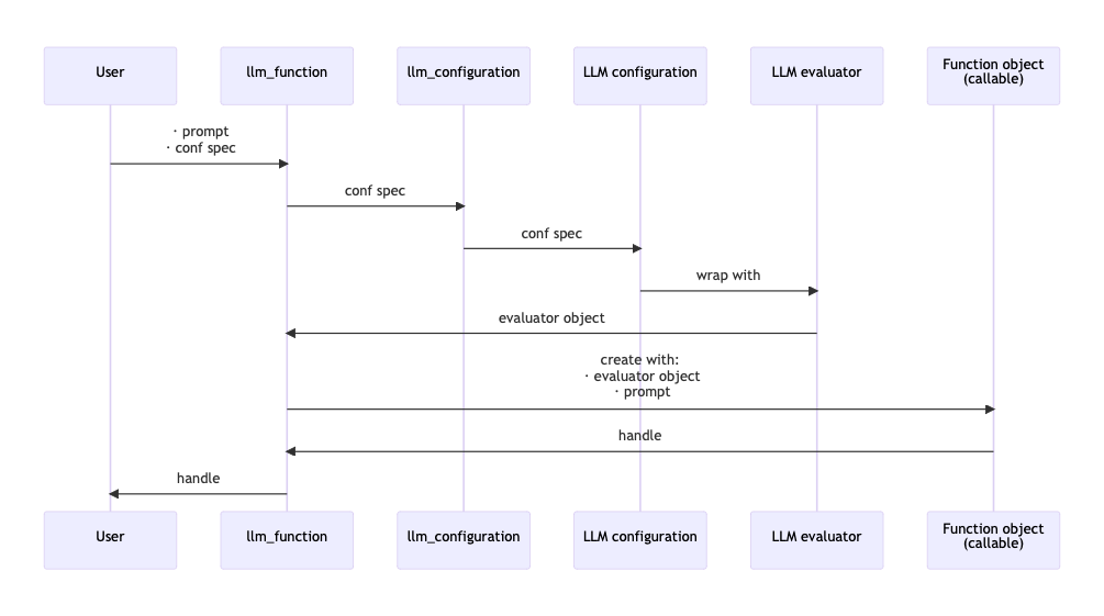
Here is a sequence diagram that follows the steps of a typical creation procedure of LLM configuration- and evaluator objects, and the corresponding LLM-function that utilizes them:

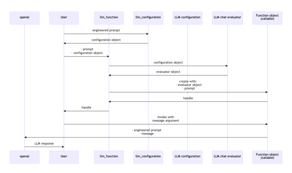
Here is a sequence diagram for making a LLM configuration with a global (engineered) prompt, and using that configuration to generate a chat message response:


Configurations

OpenAI-based

Here is the default, OpenAI-based configuration:

from LLMFunctionObjects import * for k, v in llm_configuration('OpenAI').to_dict().items(): print(f"{k} : {repr(v)}")

name : 'openai'
api_key : None
api_user_id : 'user'
module : 'openai'
model : 'gpt-3.5-turbo-instruct'
function : <bound method Completion.create of <class 'openai.api_resources.completion.Completion'>>
temperature : 0.2
total_probability_cutoff : 0.03
max_tokens : 300
fmt : 'values'
prompts : []
prompt_delimiter : ' '
stop_tokens : None
tools : []
tool_prompt : ''
tool_request_parser : None
tool_response_insertion_function : None
argument_renames : {}
evaluator : None
known_params : ['api_key', 'model', 'prompt', 'suffix', 'max_tokens', 'temperature', 'top_p', 'n', 'stream', 'logprobs', 'stop', 'presence_penalty', 'frequency_penalty', 'best_of', 'logit_bias', 'user']
response_object_attribute : None
response_value_keys : ['choices', 0, 'text']
llm_evaluator : <class 'LLMFunctionObjects.Evaluator.Evaluator'>

Here is the ChatGPT-based configuration:

for k, v in llm_configuration('ChatGPT').to_dict().items(): print(f"{k} : {repr(v)}")

name : 'chatgpt'
api_key : None
api_user_id : 'user'
module : 'openai'
model : 'gpt-3.5-turbo-0613'
function : <bound method ChatCompletion.create of <class 'openai.api_resources.chat_completion.ChatCompletion'>>
temperature : 0.2
total_probability_cutoff : 0.03
max_tokens : 300
fmt : 'values'
prompts : []
prompt_delimiter : ' '
stop_tokens : None
tools : []
tool_prompt : ''
tool_request_parser : None
tool_response_insertion_function : None
argument_renames : {}
evaluator : None
known_params : ['api_key', 'model', 'messages', 'functions', 'function_call', 'temperature', 'top_p', 'n', 'stream', 'logprobs', 'stop', 'presence_penalty', 'frequency_penalty', 'logit_bias', 'user']
response_object_attribute : None
response_value_keys : ['choices', 0, 'message', 'content']
llm_evaluator : <class 'LLMFunctionObjects.EvaluatorChatGPT.EvaluatorChatGPT'>

Remark: llm_configuration(None) is equivalent to llm_configuration('OpenAI').

Remark: Both the “OpenAI” and “ChatGPT” configuration use functions of the package “openai”, [OAIp1]. The “OpenAI” configuration is for text-completions; the “ChatGPT” configuration is for chat-completions.

PaLM-based

Here is the default PaLM configuration:

for k, v in llm_configuration('PaLM').to_dict().items(): print(f"{k} : {repr(v)}")

name : 'palm'
api_key : None
api_user_id : 'user'
module : 'google.generativeai'
model : 'models/text-bison-001'
function : <function generate_text at 0x10a04b6d0>
temperature : 0.2
total_probability_cutoff : 0.03
max_tokens : 300
fmt : 'values'
prompts : []
prompt_delimiter : ' '
stop_tokens : None
tools : []
tool_prompt : ''
tool_request_parser : None
tool_response_insertion_function : None
argument_renames : {}
evaluator : None
known_params : ['model', 'prompt', 'temperature', 'candidate_count', 'max_output_tokens', 'top_p', 'top_k', 'safety_settings', 'stop_sequences', 'client']
response_object_attribute : 'result'
response_value_keys : []
llm_evaluator : <class 'LLMFunctionObjects.Evaluator.Evaluator'>


Basic usage of LLM functions

Textual prompts

Here we make a LLM function with a simple (short, textual) prompt:

func = llm_function('Show a recipe for:')

Here we evaluate over a message:

print(func('greek salad'))

Greek Salad Recipe:

Ingredients:
- 1 large cucumber, diced
- 2 large tomatoes, diced
- 1 red onion, thinly sliced
- 1 green bell pepper, diced
- 1/2 cup Kalamata olives, pitted and halved
- 1/2 cup crumbled feta cheese
- 1/4 cup extra virgin olive oil
- 2 tablespoons red wine vinegar
- 1 teaspoon dried oregano
- Salt and pepper to taste

Instructions:

1. In a large bowl, combine the diced cucumber, tomatoes, red onion, bell pepper, and Kalamata olives.

2. In a small bowl, whisk together the olive oil, red wine vinegar, dried oregano, and salt and pepper.

3. Pour the dressing over the vegetables and toss to combine.

4. Sprinkle the crumbled feta cheese over the top of the salad.

5. Serve immediately or refrigerate until ready to serve.

Optional: You can also add some chopped fresh herbs, such as parsley or dill, for extra flavor and freshness. Enjoy your delicious and refreshing Greek salad!

Positional arguments

Here we make a LLM function with a function-prompt and numeric interpreter of the result:

func2 = llm_function( lambda a, b: f"How many {a} can fit inside one {b}?", form=float, llm_evaluator='palm')

Here were we apply the function:

res2 = func2("tennis balls", "toyota corolla 2010") res2

350.0

Here we show that we got a number:

type(res2)

float

Named arguments

Here the first argument is a template with two named arguments:

func3 = llm_function(lambda dish, cuisine: f"Give a recipe for {dish} in the {cuisine} cuisine.", llm_evaluator='palm')

Here is an invocation:

print(func3(dish='salad', cuisine='Russian', max_tokens=300))

**Ingredients:**

* 1 head of cabbage, shredded
* 1 carrot, grated
* 1/2 cup of peas, cooked
* 1/2 cup of chopped walnuts
* 1/2 cup of mayonnaise
* 1/4 cup of sour cream
* Salt and pepper to taste

**Instructions:**

1. In a large bowl, combine the cabbage, carrots, and peas.
2. In a small bowl, whisk together the mayonnaise, sour cream, salt, and pepper.
3. Pour the dressing over the salad and toss to coat.
4. Serve immediately or chill for later.

**Tips:**

* For a more flavorful salad, add some chopped fresh herbs, such as dill or parsley.
* You can also add some chopped red onion or celery to the salad.
* If you don't have any peas on hand, you can use green beans or corn instead.
* The dressing can be made ahead of time and stored in the refrigerator. Just be sure to bring it to room temperature before using it to dress the salad.


LLM example functions

The function llm_example_function can be given a training set of examples in order to generating results according to the “laws” implied by that training set.

Here a LLM is asked to produce a generalization:

llm_example_function({'finger': 'hand', 'hand': 'arm'})('foot')

' leg'

Here is an array of training pairs is used:

llm_example_function({"Einstein": "14 March 1879", "Pauli": "April 25, 1900"})('Oppenheimer')

' April 22, 1904'

Here is defined a LLM function for translating WL associations into Python dictionaries:

fea = llm_example_function(('<| A->3, 4->K1 |>', '{ A:3, 4:K1 }')) print(fea('<| 23->3, G->33, T -> R5|>'))

 { 23:3, G:33, T:R5 }

The function llm_example_function takes as a first argument:

  • Single tuple object of two scalars
  • dict
  • list object of pairs (tuple objects)

Remark: The function llm_example_function is implemented with llm_function and suitable prompt.

Here is an example of using hints:

fec = llm_example_function( {"crocodile" : "grasshopper", "fox" : "cardinal"}, hint = 'animal colors') print(fec('raccoon'))

 cardinal

Synthesizing responses

Here is an example of prompt synthesis with the function llm_synthesize using prompts from the package “LLMPrompts”, [AAp8]:

from LLMPrompts import * print( llm_synthesize([ llm_prompt("Yoda"), "Hi! How old are you?", llm_prompt("HaikuStyled") ]))

Young or old, matters not
Age is just a number, hmm
The Force is with me.


Using chat-global prompts

The configuration objects can be given prompts that influence the LLM responses “globally” throughout the whole chat. (See the second sequence diagram above.)


Chat objects

Here we create chat object that uses OpenAI’s ChatGPT:

prompt = "You are a gem expert and you give concise answers." chat = llm_chat(prompt = prompt, chat_id = 'gem-expert-talk', conf = 'ChatGPT')

chat.eval('What is the most transparent gem?')

'The most transparent gem is diamond.'

chat.eval('Ok. What are the second and third most transparent gems?')

'The second most transparent gem is sapphire, and the third most transparent gem is emerald.'

Here are the prompt(s) and all messages of the chat object:

chat.print()

Chat ID: gem-expert-talk
------------------------------------------------------------
Prompt:
You are a gem expert and you give concise answers.
------------------------------------------------------------
{'role': 'user', 'content': 'What is the most transparent gem?', 'timestamp': 1695699574.024279}
------------------------------------------------------------
{'role': 'assistant', 'content': 'The most transparent gem is diamond.', 'timestamp': 1695699575.158463}
------------------------------------------------------------
{'role': 'user', 'content': 'Ok. What are the second and third most transparent gems?', 'timestamp': 1695699588.455979}
------------------------------------------------------------
{'role': 'assistant', 'content': 'The second most transparent gem is sapphire, and the third most transparent gem is emerald.', 'timestamp': 1695699589.6835861}


References

Articles

[AA1] Anton Antonov, “Generating documents via templates and LLMs”, (2023), RakuForPrediction at WordPress.

[ZG1] Zoubin Ghahramani, “Introducing PaLM 2”, (2023), Google Official Blog on AI.

Repositories, sites

[OAI1] OpenAI Platform, OpenAI platform.

[WRIr1] Wolfram Research, Inc. Wolfram Prompt Repository.

Packages, paclets

[AAp1] Anton Antonov, LLM::Functions Raku package, (2023), GitHub/antononcube.

[AAp2] Anton Antonov, WWW::OpenAI Raku package, (2023), GitHub/antononcube.

[AAp3] Anton Antonov, WWW::PaLM Raku package, (2023), GitHub/antononcube.

[AAp4] Anton Antonov, Text::SubParsers Raku package, (2023), GitHub/antononcube.

[AAp5] Anton Antonov, Text::CodeProcessing Raku package, (2021), GitHub/antononcube.

[AAp6] Anton Antonov, ML::FindTextualAnswer Raku package, (2023), GitHub/antononcube.

[AAp7] Anton Antonov, ML::NLPTemplateEngine Raku package, (2023), GitHub/antononcube.

[AAp8] Anton Antonov, LLMPrompts Python package, (2023), PyPI.org/antononcube.

[GAIp1] Google AI, google-generativeai (Google Generative AI Python Client), (2023), PyPI.org/google-ai.

[OAIp1] OpenAI, openai (OpenAI Python Library), (2020-2023), PyPI.org.

[WRIp1] Wolfram Research, Inc. LLMFunctions paclet, (2023), Wolfram Language Paclet Repository.

DataTypeSystem


This blog post proclaims and briefly describes the Python package “DataTypeSystem” that provides a type system for different data structures that are coercible into full arrays. The package is a Python translation of the Raku package “Data::TypeSystem”, [AAp1].

Installation

Install from GitHub

pip install -e git+https://github.com/antononcube/Python-packages.git#egg=DataTypeSystem-antononcube\&subdirectory=DataTypeSystem

From PyPi

pip install DataTypeSystem


Usage examples

The type system conventions follow those of Mathematica’s Dataset — see the presentation “Dataset improvements”.

Here we get the Titanic dataset, change the “passengerAge” column values to be numeric, and show dataset’s dimensions:

import pandas dfTitanic = pandas.read_csv('https://raw.githubusercontent.com/mwaskom/seaborn-data/master/titanic.csv') dfTitanic = dfTitanic[["sex", "age", "pclass", "survived"]] dfTitanic = dfTitanic.rename(columns ={"pclass": "class"}) dfTitanic.shape

(891, 4)

Here is a sample of dataset’s records:

from DataTypeSystem import * dfTitanic.sample(3)

sexageclasssurvived
555male62.010
278male7.030
266male16.030

Here is the type of a single record:

deduce_type(dfTitanic.iloc[12].to_dict())

Struct([age, class, sex, survived], [float, int, str, int])

Here is the type of single record’s values:

deduce_type(dfTitanic.iloc[12].to_dict().values())

Tuple([Atom(<class 'str'>), Atom(<class 'float'>), Atom(<class 'int'>), Atom(<class 'int'>)])

Here is the type of the whole dataset:

deduce_type(dfTitanic.to_dict())

Assoc(Atom(<class 'str'>), Assoc(Atom(<class 'int'>), Atom(<class 'str'>), 891), 4)

Here is the type of “values only” records:

valArr = dfTitanic.transpose().to_dict().values() deduce_type(valArr)

Vector(Struct([age, class, sex, survived], [float, int, str, int]), 891)


References

[AAp1] Anton Antonov, Data::TypeSystem Raku package, (2023), GitHub/antononcube.

Tries with frequencies

Introduction

This blog post introduces and gives usage examples of the Machine Learning (ML) data structure Tries with frequencies, [AA1], creation and usage through the Python package “TriesWithFrequencies”.

For the original Trie (or Prefix tree) data structure see the Wikipedia article “Trie”.


Setup

from TriesWithFrequencies import *

Creation examples

In this section we show a few ways to create tries with frequencies.

Consider a trie (prefix tree) created over a list of words:

tr = trie_create_by_split( ["bar", "bark", "bars", "balm", "cert", "cell"] )
trie_form(tr)
TRIEROOT => 6.0
├─b => 4.0
│ └─a => 4.0
│   ├─r => 3.0
│   │ └─k => 1.0
│   │ └─s => 1.0
│   └─l => 1.0
│     └─m => 1.0
└─c => 2.0
  └─e => 2.0
    ├─r => 1.0
    │ └─t => 1.0
    └─l => 1.0
      └─l => 1.0

Here we convert the trie with frequencies above into a trie with probabilities:

ptr = trie_node_probabilities( tr )
trie_form(ptr)
TRIEROOT => 1.0
├─b => 0.6666666666666666
│ └─a => 1.0
│   ├─r => 0.75
│   │ ├─k => 0.3333333333333333
│   │ └─s => 0.3333333333333333
│   └─l => 0.25
│     └─m => 1.0
└─c => 0.3333333333333333
  └─e => 1.0
    ├─r => 0.5
    │ └─t => 1.0
    └─l => 0.5
      └─l => 1.0


Shrinking

Here we shrink the trie with probabilities above:

trie_form(trie_shrink(ptr))
TRIEROOT => 1.0
└─ba => 1.0
  └─r => 0.75
    └─k => 0.3333333333333333
    └─s => 0.3333333333333333
  └─lm => 1.0
└─ce => 1.0
  └─rt => 1.0
  └─ll => 1.0

Here we shrink the frequencies trie using a separator:

trie_form(trie_shrink(tr, sep="~"))
TRIEROOT => 6.0
└─b~a => 4.0
  └─r => 3.0
    └─k => 1.0
    └─s => 1.0
  └─l~m => 1.0
└─c~e => 2.0
  └─r~t => 1.0
  └─l~l => 1.0


Retrieval and sub-tries

Here we retrieve a sub-trie with a key:

trie_form(trie_sub_trie(tr, list("bar")))
r => 3.0
└─k => 1.0
└─s => 1.0


Classification

Create a trie:

words = [*(["bar"] * 6), *(["bark"] * 3), *(["bare"] * 2), *(["cam"] * 3), "came", *(["camelia"] * 4)]
tr = trie_create_by_split(words)
tr = trie_node_probabilities(tr)

Show node counts:

trie_node_counts(tr)
{'total': 13, 'internal': 10, 'leaves': 3}

Show the trie form:

trie_form(tr)
TRIEROOT => 1.0
├─b => 0.5789473684210527
│ └─a => 1.0
│   └─r => 1.0
│     ├─k => 0.2727272727272727
│     └─e => 0.18181818181818182
└─c => 0.42105263157894735
  └─a => 1.0
    └─m => 1.0
      └─e => 0.625
        └─l => 0.8
          └─i => 1.0
            └─a => 1.0

Classify with the letters of the word \”cam\”:

trie_classify(tr, list("cam"), prop="Probabilities")
{'a': 0.5, 'm': 0.375, 'e': 0.12499999999999997}


References

Articles

[AA1] Anton Antonov, “Tries with frequencies for data mining”, (2013), MathematicaForPrediction at WordPress.

[AA2] Anton Antonov, “Removal of sub-trees in tries”, (2013), MathematicaForPrediction at WordPress.

[AA3] Anton Antonov, “Tries with frequencies in Java” (2017), MathematicaForPrediction at WordPressGitHub Markdown.

[WK1] Wikipedia entry, Trie.

Packages

[AAp1] Anton Antonov, Tries with frequencies Mathematica Version 9.0 package, (2013), MathematicaForPrediction at GitHub.

[AAp2] Anton Antonov, Tries with frequencies Mathematica package, (2013-2018), MathematicaForPrediction at GitHub.

[AAp3] Anton Antonov, Tries with frequencies in Java, (2017), MathematicaForPrediction at GitHub.

[AAp4] Anton Antonov, Java tries with frequencies Mathematica package, (2017), MathematicaForPrediction at GitHub.

[AAp5] Anton Antonov, Java tries with frequencies Mathematica unit tests, (2017), MathematicaForPrediction at GitHub.

[AAp6] Anton Antonov, ML::TriesWithFrequencies Raku package, (2021), GitHub/antononcube.

Videos

[AAv1] Anton Antonov, “Prefix Trees with Frequencies for Data Analysis and Machine Learning”, (2017), Wolfram Technology Conference 2017, Wolfram channel at YouTube.

Stand-alone ROC functions package

This blog post proclaims and outlines the usage of the Python package “ROCFunctions” that provides Receiver Operating Characteristic (ROC) functions.

The ROC framework is used for analysis and tuning of binary classifiers, [Wk1]. (The classifiers are assumed to classify into a positive/true label or a negative/false label. )

For computational introduction to ROC utilization (in Mathematica) see the article “Basic example of using ROC with Linear regression” , [AA1].

The examples below use the package “RandomDataGenerators”, [AA2].

Remark: Different classification-related Python packages provide ROC functions, but all of them — well, the ones I tried — have a certain opinionated signatures and workflow of usage. I think it is a very good idea to have a stand-alone package that is independent of other packages, and, hence, it is applicable in all cases.


Installation

From PyPI.org:

python3 -m pip install ROCFunctions

Usage examples

Properties

Here are some retrieval functions:

import pandas
from ROCFunctions import *
print(roc_functions("properties"))
['FunctionInterpretations', 'FunctionNames', 'Functions', 'Methods', 'Properties']
print(roc_functions("FunctionInterpretations"))
{'TPR': 'true positive rate', 'TNR': 'true negative rate', 'SPC': 'specificity', 'PPV': 'positive predictive value', 'NPV': 'negative predictive value', 'FPR': 'false positive rate', 'FDR': 'false discovery rate', 'FNR': 'false negative rate', 'ACC': 'accuracy', 'AUROC': 'area under the ROC curve', 'FOR': 'false omission rate', 'F1': 'F1 score', 'MCC': 'Matthews correlation coefficient', 'Recall': 'same as TPR', 'Precision': 'same as PPV', 'Accuracy': 'same as ACC', 'Sensitivity': 'same as TPR'}
print(roc_functions("FPR"))
<function FPR at 0x12a9fe050>

Single ROC record

Definition: A ROC record (ROC-dictionary, or ROC-hash, or ROC-hash-map) is an associative object that has the keys: “FalseNegative”, “FalsePositive”, “TrueNegative”, “TruePositive”.Here is an example:

{"FalseNegative": 50, "FalsePositive": 51, "TrueNegative": 60, "TruePositive": 39}
{'FalseNegative': 50,
 'FalsePositive': 51,
 'TrueNegative': 60,
 'TruePositive': 39}

Here we generate a random “dataset” with columns “Actual” and “Predicted” that have the values “true” and “false”and show the summary:

from RandomDataGenerators import *

dfRandomLabels = random_data_frame(200, ["Actual", "Predicted"],
                                   generators={"Actual": ["true", "false"],
                                               "Predicted": ["true", "false"]})
dfRandomLabels.shape
(200, 2)

Here is a sample of the dataset:

print(dfRandomLabels[:4])
  Actual Predicted
0  false      true
1   true     false
2   true      true
3   true     false

Here we make the corresponding ROC dictionary:

to_roc_dict('true', 'false',
            list(dfRandomLabels.Actual.values),
            list(dfRandomLabels.Predicted.values))
{'TruePositive': 46,
 'FalsePositive': 52,
 'TrueNegative': 53,
 'FalseNegative': 49}

Multiple ROC records

Here we make random dataset with entries that associated with a certain threshold parameter with three unique values:

dfRandomLabels2 = random_data_frame(200, ["Threshold", "Actual", "Predicted"],
                                    generators={"Threshold": [0.2, 0.4, 0.6],
                                                "Actual": ["true", "false"],
                                                "Predicted": ["true", "false"]})

Remark: Threshold parameters are typically used while tuning Machine Learning (ML) classifiers. Here we find and print the ROC records(dictionaries) for each unique threshold value:

thresholds = list(dfRandomLabels2.Threshold.drop_duplicates())

rocGroups = {}
for x in thresholds:
    dfLocal = dfRandomLabels2[dfRandomLabels2["Threshold"] == x]
    rocGroups[x] = to_roc_dict('true', 'false',
                        list(dfLocal.Actual.values),
                        list(dfLocal.Predicted.values))

rocGroups
{0.2: {'TruePositive': 19,
  'FalsePositive': 18,
  'TrueNegative': 13,
  'FalseNegative': 13},
 0.4: {'TruePositive': 23,
  'FalsePositive': 20,
  'TrueNegative': 19,
  'FalseNegative': 17},
 0.6: {'TruePositive': 20,
  'FalsePositive': 10,
  'TrueNegative': 9,
  'FalseNegative': 19}}

Application of ROC functions

Here we define a list of ROC functions:

funcs = ["PPV", "NPV", "TPR", "ACC", "SPC", "MCC"]

Here we apply each ROC function to each of the ROC records obtained above:

import pandas
rocRes = { k : {f: roc_functions(f)(v) for f in funcs} for (k, v) in rocGroups.items()}

print(pandas.DataFrame(rocRes))
          0.2       0.4       0.6
PPV  0.513514  0.534884  0.666667
NPV  0.500000  0.527778  0.321429
TPR  0.593750  0.575000  0.512821
ACC  0.507937  0.531646  0.500000
SPC  0.419355  0.487179  0.473684
MCC  0.013309  0.062421 -0.013506

References

Articles

[Wk1] Wikipedia entry, “Receiver operating characteristic”.

[AA1] Anton Antonov, “Basic example of using ROC with Linear regression” , (2016), MathematicaForPrediction at WordPress.

[AA2] Anton Antonov, “Introduction to data wrangling with Raku” , (2021), RakuForPrediction at WordPress.

Packages

[AAp1] Anton Antonov, ROCFunctions Mathematica package, (2016-2022), MathematicaForPrediction at GitHub/antononcube.

[AAp2] Anton Antonov, ROCFunctions R package, (2021), R-packages at GitHub/antononcube.

[AAp3] Anton Antonov, ML::ROCFunctions Raku package, (2022), GitHub/antononcube.

Example datasets retrieval

This blog post proclaims and briefly describes the Python package “ExampleDatasets” for (obtaining) example datasets.

Currently, this repository contains only datasets metadata. The datasets are downloaded from the repository Rdatasets, [VAB1].

This package follows the design of the Raku package “Data::ExampleDatasets”; see [AAr1].


Usage examples

Setup

Here we load the Python packages timepandas, and this package:

from ExampleDatasets import *
import pandas

Get a dataset by using an identifier

Here we get a dataset by using an identifier and display part of the obtained dataset:

tbl = example_dataset(itemSpec = 'Baumann')
tbl.head
<bound method NDFrame.head of     Unnamed: 0  group  pretest.1  pretest.2  post.test.1  post.test.2  \
0            1  Basal          4          3            5            4   
1            2  Basal          6          5            9            5   
2            3  Basal          9          4            5            3   
3            4  Basal         12          6            8            5   
4            5  Basal         16          5           10            9   
..         ...    ...        ...        ...          ...          ...   
61          62  Strat         11          4           11            7   
62          63  Strat         14          4           15            7   
63          64  Strat          8          2            9            5   
64          65  Strat          5          3            6            8   
65          66  Strat          8          3            4            6   

    post.test.3  
0            41  
1            41  
2            43  
3            46  
4            46  
..          ...  
61           48  
62           49  
63           33  
64           45  
65           42  

[66 rows x 7 columns]>

Here we summarize the dataset obtained above:

tbl.describe()
Unnamed: 0pretest.1pretest.2post.test.1post.test.2post.test.3
count66.00000066.00000066.00000066.00000066.00000066.000000
mean33.5000009.7878795.1060618.0757586.71212144.015152
std19.1963543.0205202.2127523.3937072.6356446.643661
min1.0000004.0000001.0000001.0000000.00000030.000000
25%17.2500008.0000003.2500005.0000005.00000040.000000
50%33.5000009.0000005.0000008.0000006.00000045.000000
75%49.75000012.0000006.00000011.0000008.00000049.000000
max66.00000016.00000013.00000015.00000013.00000057.000000

Remark: The values for the arguments itemSpec and packageSpec correspond to the values of the columns “Item” and “Package”, respectively, in the metadata dataset from the GitHub repository “Rdatasets”, [VAB1]. See the datasets metadata sub-section below.

Get a dataset by using an URL

Here we can find URLs of datasets that have titles adhering to a regex:

dfMeta = load_datasets_metadata()
print(dfMeta[dfMeta.Title.str.contains('^tita')][["Package", "Item", "CSV"]].to_string())
    Package        Item                                                                      CSV
288 COUNT titanic https://vincentarelbundock.github.io/Rdatasets/csv/COUNT/titanic.csv
289 COUNT titanicgrp https://vincentarelbundock.github.io/Rdatasets/csv/COUNT/titanicgrp.csv

Here we get a dataset through pandas by using an URL and display the head of the obtained dataset:

import pandas
url = 'https://raw.githubusercontent.com/antononcube/Raku-Data-Reshapers/main/resources/dfTitanic.csv'
tbl2 = pandas.read_csv(url)
tbl2.head()
idpassengerClasspassengerAgepassengerSexpassengerSurvival
011st30femalesurvived
121st0malesurvived
231st0femaledied
341st30maledied
451st20femaledied

Datasets metadata

Here we:

  1. Get the dataset of the datasets metadata
  2. Filter it to have only datasets with 13 rows
  3. Keep only the columns “Item”, “Title”, “Rows”, and “Cols”
  4. Display it
tblMeta = load_datasets_metadata()
tblMeta = tblMeta[["Item", "Title", "Rows", "Cols"]]
tblMeta = tblMeta[tblMeta["Rows"] == 13]
tblMeta
ItemTitleRowsCols
805Snow.pumpsJohn Snow’s Map and Data on the 1854 London Ch…134
820BCGBCG Vaccine Data137
935cementHeat Evolved by Setting Cements135
1354kootenayWaterflow Measurements of Kootenay River in Li…132
1644Newhouse77Medical-Care Expenditure: A Cross-National Sur…135
1735SaxonyFamilies in Saxony132

Keeping downloaded data

By default the data is obtained over the web from Rdatasets, but example_dataset has an option to keep the data “locally.” (The data is saved in XDG_DATA_HOME, see SS1.)

This can be demonstrated with the following timings of a dataset with ~1300 rows:

import time
startTime = time.time()
data = example_dataset(itemSpec = 'titanic', packageSpec = 'COUNT', keep = True)
endTime = time.time()
print("Getting the data first time took " + str( endTime - startTime ) + " seconds")
Getting the data first time took 0.003923892974853516 seconds
import time
startTime = time.time()
data = example_dataset(itemSpec = 'titanic', packageSpec = 'COUNT', keep = True)
endTime = time.time()
print("Geting the data second time took " + str( endTime - startTime ) + " seconds")
Geting the data second time took 0.003058910369873047 seconds

References

Functions, packages, repositories

[AAf1] Anton Antonov, ExampleDataset, (2020), Wolfram Function Repository.

[AAr1] Anton Antonov, Data::ExampleDatasets Raku package, (2021), GitHub/antononcube.

[VAB1] Vincent Arel-Bundock, Rdatasets, (2020), GitHub/vincentarelbundock.

[SS1] Scott Stevenson, xdg Python package, (2016-2021), PyPI.org.

Interactive interfaces

[AAi1] Anton Antonov, Example datasets recommender interface, (2021), Shinyapps.io.

Facing data with Chernoff faces

Introduction

This blog post proclaims the Python package “ChernoffFace” and outlines and exemplifies its function chernoff_face that generates Chernoff diagrams.

The design, implementation strategy, and unit tests closely resemble the Wolfram Repository Function (WFR) ChernoffFace, [AAf1], and the original Mathematica package “ChernoffFaces.m”, [AAp1].


Installation

To install from GitHub use the shell command:

python -m pip install git+https://github.com/antononcube/Python-packages.git#egg=ChernoffFace\&subdirectory=ChernoffFace

To install from PyPI:

python -m pip install ChernoffFace


Usage examples

Setup

from ChernoffFace import *
import numpy
import matplotlib.cm

Random data

# Generate data
numpy.random.seed(32)
data = numpy.random.rand(16, 12)
# Make Chernoff faces
fig = chernoff_face(data=data,
                    titles=[str(x) for x in list(range(len(data)))],
                    color_mapper=matplotlib.cm.Pastel1)
png

Employee attitude data

Get Employee attitude data

dfData=load_employee_attitude_data_frame()
dfData.head()
RatingComplaintsPrivilegesLearningRaisesCriticalAdvancement
043513039619245
163645154637347
271706869768648
361634547548435
481785666718347

Rescale the variables:

dfData2 = variables_rescale(dfData)
dfData2.head()
RatingComplaintsPrivilegesLearningRaisesCriticalAdvancement
00.0666670.2641510.0000000.1219510.4000001.0000000.425532
10.5111110.5094340.3962260.4878050.4444440.5581400.468085
20.6888890.6226420.7169810.8536590.7333330.8604650.489362
30.4666670.4905660.2830190.3170730.2444440.8139530.212766
40.9111110.7735850.4905660.7804880.6222220.7906980.468085

Make the corresponding Chernoff faces:

fig = chernoff_face(data=dfData2,
                    n_columns=5,
                    long_face=False,
                    color_mapper=matplotlib.cm.tab20b,
                    figsize=(8, 8), dpi=200)
png

USA arrests data

Get USA arrests data:

dfData=load_usa_arrests_data_frame()
dfData.head()
StateNameMurderAssaultUrbanPopulationRape
0Alabama13.22365821.2
1Alaska10.02634844.5
2Arizona8.12948031.0
3Arkansas8.81905019.5
4California9.02769140.6

Rescale the variables:

dfData2 = variables_rescale(dfData)
dfData2.head()
StateNameMurderAssaultUrbanPopulationRape
0Alabama0.7469880.6541100.4406780.359173
1Alaska0.5542170.7465750.2711860.961240
2Arizona0.4397590.8527400.8135590.612403
3Arkansas0.4819280.4965750.3050850.315245
4California0.4939760.7910961.0000000.860465

Make the corresponding Chernoff faces using USA state names as titles:

fig = chernoff_face(data=dfData2,
                    n_columns=5,
                    long_face=False,
                    color_mapper=matplotlib.cm.tab20c_r,
                    figsize=(12, 12), dpi=200)
png

References

Articles

[AA1] Anton Antonov, “Making Chernoff faces for data visualization”, (2016), MathematicaForPrediction at WordPress.

Functions and packages

[AAf1] Anton Antonov, ChernoffFace, (2019), Wolfram Function Repository.

[AAp1] Anton Antonov, Chernoff faces implementation in Mathematica, (2016), MathematicaForPrediction at GitHub.

Random Mandalas Generator

Introduction

This blog post proclaims the Python package “RandomMandala” and fully describes its function random_mandala that generates plots (and images) of random mandalas.

The design, implementation strategy, and unit tests closely resemble the Wolfram Repository Function (WFR) RandomMandala, [AAf1].

(Another, very similar function at WFR is RandomScribble, [AAf2].)

The Bezier mandala seeds are created using the Python package bezier, [DHp1].

For detailed descriptions of Machine Learning studies that use collections of random mandalas see the articles [AA1, AA2] and related presentation [AAv1].

Remark: This Markdown file was automatically generated from the notebook: “RandomMandala-package.ipynb”.


Installation

To install from GitHub use the shell command:

python -m pip install git+https://github.com/antononcube/Python-packages.git#egg=RandomMandala\&subdirectory=RandomMandala

To install from PyPI:

python -m pip install RandomMandala

Details and arguments

  • The mandalas made by random_mandala are generated through rotational symmetry of a “seed segment”.
  • The function random_mandala returns matplotlib figures (objects of type matplotlib.figure.Figure)
  • The function random_mandala can be given arguments of the creation function matplotlib.pyplot.figure.
  • If n_rows and n_columns are None a matplotlib figure object with one axes object is returned.
  • There are two modes of making random mandalas: (i) single-mandala mode and (ii) multi-mandala mode. The multi-mandala mode is activated by giving the radius argument a list of positive numbers.
  • If the argument radius is a list of positive reals, then a “multi-mandala” is created with the mandalas corresponding to each number in the radius list being overlain.
  • Here are brief descriptions of the arguments:
    • n_rows: Number of rows in the result figure.
    • n_columns: Number of columns in the result figure.
    • radius: Radius for the mandalas, a flot or a list of floats. If a list of floats the mandalas are overlain.
    • rotational_symmetry_order: Number of copies of the seed segment that comprise the mandala.
    • connecting_function: Connecting function, one of “line”, “fill”, “bezier”, “bezier_fill”, “random”, or None. If ‘random’ or None a random choice of the rest of values is made.
    • number_of_elements: Controls how may graphics elements are in the seed segment.
    • symmetric_seed: Specifies should the seed segment be symmetric or not. If ‘random’ of None random choice between True and False is made.
    • face_color: Face (fill) color.
    • edge_color: Edge (line) color.

Examples

Load the package RandomMandalamatplotlib, and PIL:

from RandomMandala import random_mandala, figure_to_image
import matplotlib
import matplotlib.pyplot as plt
import matplotlib.cm
from PIL import Image, ImageOps
from mpl_toolkits.axes_grid1 import ImageGrid
import random

Here we generate a random mandala:

random.seed(99)
fig = random_mandala()
png

Here we generate a figure with 12 (3×4) random mandalas:

random.seed(33)
fig2 = random_mandala(n_rows=3, n_columns=4, figsize=(6,6))
fig2.tight_layout()
plt.show()
png

Arguments details

n_rows, n_columns

With the argument n_rows and n_columns are specified the number of rows and columns respectively in the figure object; n_rows * n_columns mandalas are generated:

random.seed(22)
fig=random_mandala(n_rows=1, n_columns=3)
png

connecting_function

The argument connecting_function specifies which graphics primitives to be used over the seed segment points:

fig = matplotlib.pyplot.figure(figsize=(6, 6), dpi=120)

k = 1
for cf in ['line', 'fill', 'bezier', 'bezier_fill', 'random', None]:
    random.seed(667)
    fig = random_mandala(connecting_function=cf,
                         figure=fig,
                         location=(2, 3, k))
    ax = fig.axes[-1]
    ax.set_title(str(cf))
    k = k + 1
plt.show()
plt.close(fig)
png

With values None or "random" a random choice is made from ['line', 'fill', 'bezier', 'bezier_fill'].

radius

In single-mandala mode the argument radius specifies the radius of the seed segment and the mandala:

fig = matplotlib.pyplot.figure(figsize=(8, 4), dpi=120)
k = 1
for r in [5, 10, 15, 20]:
    random.seed(2)
    fig = random_mandala(connecting_function="line", 
                         radius=r,
                         figure = fig,
                         location = (1, 4, k))
    ax = fig.axes[-1]
    ax.set_title("radius:" + str(r))
    ax.axis("on")
    k = k + 1
plt.show()
plt.close(fig)
png

If the value given to radius is a list of positive numbers then multi-mandala mode is used. If radius=[r[0],...,r[k]], then for each r[i] is made a mandala with radius r[i] and the mandalas are drawn upon each other according to their radii order:

random.seed(99)
fig3=random_mandala(radius=[8,5,3], 
                    face_color=["blue", "green", 'red'],
                    connecting_function="fill")                
png

Remark: The code above used different colors for the different radii.

rotational_symmetry_order

The argument rotational_symmetry_order specifies how many copies of the seed segment comprise the mandala:

fig = matplotlib.pyplot.figure(figsize=(6, 12), dpi=120)
k = 1
for rso in [2, 3, 4, 6]:
    random.seed(122)
    fig = random_mandala(connecting_function="fill", 
                         symmetric_seed=True,
                         rotational_symmetry_order=rso,
                         figure = fig,
                         location = (1, 4, k))
    ax = fig.axes[-1]
    ax.set_title("order:" + str(rso))
    k = k + 1
plt.show()
plt.close(fig)

png

number_of_elements

The argument number_of_elements controls how may graphics elements are in the seed segment:

fig = matplotlib.pyplot.figure(figsize=(6, 6), dpi=120)
k = 1
for ne in [2, 3, 4, 5, 6, 12]:
    random.seed(2)
    fig = random_mandala(connecting_function="line",
                         symmetric_seed=True,
                         rotationa_symmetry_order=6,
                         number_of_elements=ne,
                         figure = fig,
                         location = (2, 3, k))
    ax = fig.axes[-1]
    ax.set_title("n:" + str(ne))
    k = k + 1
plt.show()
plt.close(fig)
png
fig = matplotlib.pyplot.figure(figsize=(4, 4), dpi=120)
k = 1
for ne in [5, 10, 15, 20]:
    random.seed(26)
    fig = random_mandala(connecting_function="bezier",
                         radius=[1],
                         symmetric_seed=True,
                         rotationa_symmetry_order=6,
                         number_of_elements=ne,
                         figure = fig,
                         location = (2, 2, k))
    ax = fig.axes[-1]
    ax.set_title("n:" + str(ne))
    k = k + 1
plt.show()
plt.close(fig)
png

symmetric_seed

The argument symmetric_seed specifies should the seed segment be symmetric or not:

fig = matplotlib.pyplot.figure(figsize=(4, 4), dpi=120)
k = 1
for ssd in [True, False]:
    random.seed(2)
    fig = random_mandala(connecting_function="fill", 
                         symmetric_seed=ssd,
                         figure = fig,
                         location = (1, 2, k))
    ax = fig.axes[-1]
    ax.set_title(str(ssd))
    k = k + 1
plt.show()
plt.close(fig)
png

face_color and edge_color

The arguments face_color and edge_color take as values strings or list of strings that specify the coloring of the filled-in polygons and lines respectively:

fig = matplotlib.pyplot.figure(figsize=(6,3), dpi=120)
k = 1
for fc in [["0.8", "0.6", "0.2"], ["olive", "gold", "red"]]:
    random.seed(11)
    fig = random_mandala(radius=[10,6,4],
     					 connecting_function="bezier_fill", 
                         symmetric_seed=True,
                         face_color=fc,
                         figure = fig,
                         location = (1, 2, k))
    ax = fig.axes[-1]
    ax.set_title(str(fc))
    k = k + 1
    
plt.show()
plt.close(fig)
png

alpha

The argument alpha controls the opacity of the plots; it takes as values None and floats between 0 and 1.

fig = matplotlib.pyplot.figure(figsize=(6,3), dpi=120)
k = 1
for al in [None, 0.2, 1.0]:
    random.seed(23)
    fig = random_mandala(radius=[10,6,4],
     					 connecting_function="bezier_fill",
                         symmetric_seed=True,
                         alpha=al,
                         color_mapper=matplotlib.cm.rainbow_r,
                         figure = fig,
                         location = (1, 3, k))
    ax = fig.axes[-1]
    ax.set_title(str(al))
    k = k + 1

plt.show()
plt.close(fig)
png

color_mapper

The argument color_mapper takes as values None and matplotlib.colors.Colormap objects. See the color mappers in the reference page “color example code: colormaps_reference.py”. If color_mapper is specified then the arguments face_color and edge_color are ignored. Here is an example using two color mappers:

fig = matplotlib.pyplot.figure(figsize=(6,3), dpi=120)
cMappers=[matplotlib.cm.rainbow_r, matplotlib.cm.Accent_r]
cMappersNames=["rainbow_r", "Accent_r"]
for k in range(2): 
    random.seed(15)
    fig = random_mandala(radius=[10,6,4],
                         connecting_function="bezier_fill",
                         symmetric_seed=True,
                         color_mapper=cMappers[k],
                         figure = fig,
                         location = (1, 2, k+1))
    ax = fig.axes[-1]
    ax.set_title(cMappersNames[k])
    
plt.show()
plt.close(fig)
png

Applications

Generate a collection of images

In certain Machine Learning (ML) studies it can be useful to be able to generate large enough collections of (random) images.

In the code block below we:

  • Generate 64 random mandala plots
  • Convert them into PIL images using the package function figure_to_image
  • Invert and binarize images
  • Plot the images in an image grid
# A list to accumulate random mandala images
mandala_images = []

# Generation loop
random.seed(443)
for i in range(64):
    
    # Generate one random mandala figure
    fig2 = random_mandala(n_rows=None,
                          n_columns=None,
                          radius=[8, 6, 3],
                          rotational_symmetry_order=6,
                          symmetric_seed=True,
                          connecting_function='random',
                          face_color="0.")
    fig2.tight_layout()
    
    # Convert the figure into an image and add it to the list
    mandala_images = mandala_images + [figure_to_image(fig2)]
    
    # Close figure to save memoru
    plt.close(fig2)

# Invert image colors    
mandala_images2 = [ImageOps.invert(img) for img in mandala_images]

# Binarize images
mandala_images3 = [im.convert('1') for im in mandala_images2]

# Make a grid of images and display it
fig3 = plt.figure(figsize=(14., 14.))
grid = ImageGrid(fig3, 111,
                 nrows_ncols=(8, 8),
                 axes_pad=0.02,
                 )

for ax, img in zip(grid, mandala_images3):
    ax.imshow(img)
    ax.set(xticks=[], yticks=[])

plt.show()
png

Neat examples

A table of random mandalas

random.seed(124)
fig=random_mandala(n_rows=6, n_columns=6, figsize=(10,10), dpi=240)
png

A table of colorized mandalas

fig = matplotlib.pyplot.figure(figsize=(10, 10), dpi=120)
k = 1
random.seed(56)
for i in range(36):
    rs=list(range(1,random.choice([3,4,5,6])+1))
    rs.sort()
    rs.reverse()

    fig = random_mandala(connecting_function="bezier_fill",
                         color_mapper=matplotlib.cm.gist_earth,
   						 symmetric_seed=True,
                         radius=rs,
                         rotational_symmetry_order=random.choice([3,4,5,6,7]),
                         number_of_elements=random.choice([2,3,4]),
                         figure=fig,
                         location=(6, 6, k))
    ax = fig.axes[-1]
    ax.set_axis_off()
    k = k + 1

fig.tight_layout()
plt.show()
plt.close(fig)
png

A table of open colorized mandalas

fig = matplotlib.pyplot.figure(figsize=(10, 10), dpi=120)
k = 1
random.seed(883)
for rso in [2 * random.random() + 2 for _ in range(36)]:
    random.seed(33)
    fig = random_mandala(connecting_function="bezier_fill",
                         radius=3,
                         face_color="darkblue",
                         rotational_symmetry_order=rso,
                         number_of_elements=8,
                         figure=fig,
                         location=(6, 6, k))
    ax = fig.axes[-1]
    ax.set_axis_off()
    k = k + 1

plt.show()
plt.close(fig)
png

Acknowledgements


References

Articles

[AA1] Anton Antonov, “Comparison of dimension reduction algorithms over mandala images generation”, (2017), MathematicaForPrediction at WordPress.

[AA1] Anton Antonov, “Generation of Random Bethlehem Stars, (2020), MathematicaForPrediction at WordPress.

Functions

[AAf1] Anton Antonov, RandomMandala, (2019), Wolfram Function Repository.

[AAf2] Anton Antonov, RandomScribble, (2020), Wolfram Function Repository.

Packages

[DHp1] Daniel Hermes, bezier Python package, (2016), PyPy.org.

Videos

[AAv1] Anton Antonov, “Random Mandalas Deconstruction in R, Python, and Mathematica (Greater Boston useR Meetup, Feb 2022)” (2022), Anton Antonov’s channel at YouTube.

Random Sparse Matrix Generator

In brief

This blog post proclaims and briefly describes a Python package that implements the function random_sparse_matrix, which can be used to generate random sparse matrices.

The sparse matrices have named rows and columns — see the package “SSparseMatrix”, [AAp1].

Functions from the package “RandomDataGenerators”, [AAp2], are used to obtain row- and column names and entry values. (See the previous post of this blog.)


Installation

To install from GitHub use the shell command:

python -m pip install git+https://github.com/antononcube/Python-packages.git#egg=RandomSparseMatrix\&subdirectory=RandomSparseMatrix

To install from PyPI:

python -m pip install RandomSparseMatrix

Examples

Here is random sparse matrix (SSparseMatrix object) with 6 rows and 4 columns:

import random
from RandomSparseMatrix import *

random.seed(87)
rmat = random_sparse_matrix(6, 4,
                            column_names_generator=random_pet_name,
                            row_names_generator=random_word,
                            min_number_of_values=6,
                            max_number_of_values=None)
rmat.print_matrix(n_digits=20)

# ============================================================================================
#            |                Cleo             Diamond                 Max               Tessa
# --------------------------------------------------------------------------------------------
#  cuticular |                   .                   .                   .  12.886794438387263
#    elysian |                   .                   .                   .  13.891135469455826
# spot-check |                   .  11.465064963144142                   .                   .
#   cetacean |                   .   9.626463367706222                   .                   .
#       idem |   5.474873249244756                   .                   .                   .
#        lot |                   .                   .  10.818678723268317                   .
# ============================================================================================


References

[AAp1] Anton Antonov, SSparseMatrix Python package, (2021), PyPI.

[AAp2] Anton Antonov, RandomDataGenerators Python package, (2021), PyPI.

[AAp3] Anton Antonov, SparseMatrixRecommender Python package, (2021), PyPI.

Random Data Generators

Introduction

This blog post proclaims and briefly describes the Python package “RandomDataGenerators” that has functions for generating random strings, words, pet names, and (tabular) data frames.

The full list of features and development status can be found in the org-mode file Random-data-generators-work-plan.org.

Motivation

The primary motivation for this package is to have simple, intuitively named functions for generating random vectors (lists) and data frames of different objects.

Although, Python has support of random vector generation, it is assumed that commands like the following are easier to use:

random_string(6, chars = 4, pattern = "[\l\d]")


Installation

To install from GitHub use the shell command:

python -m pip install git+https://github.com/antononcube/Python-packages.git#egg=RandomDataGenerators\&subdirectory=RandomDataGenerators

To install from PyPi.org:

python -m pip install RandomDataGenerators


Setup

from RandomDataGenerators import *

The import command above is equivalent to the import commands:

from RandomDataGenerators.RandomDataFrameGenerator import random_data_frame
from RandomDataGenerators.RandomFunctions import random_string
from RandomDataGenerators.RandomFunctions import random_word
from RandomDataGenerators.RandomFunctions import random_pet_name
from RandomDataGenerators.RandomFunctions import random_pretentious_job_title

We are also going to use the packages randomnumpy, and pandas:

import random
import numpy
import pandas
pandas.set_option('display.max_columns', None)


Random strings

The function random_string generates random strings. (It is based on the package StringGenerator, \[PW1\].)

Here we generate a vector of random strings with length 4 and characters that belong to specified ranges:

random_string(6, chars=4, pattern = "[\d]") # digits only

## ['3749', '4572', '9812', '7395', '2388', '7625']

random_string(6, chars=4, pattern = "[\l]") # letters only

## ['FhSd', 'DNSu', 'YggC', 'ajqA', 'dIBt', 'Mjdc']

random_string(6, chars=4, pattern = "[\l\d]") # both digits and letters

## ['yp4u', '2Shk', 'pvpS', 'M43O', 'm5SX', 'It3L']


Random words

The function random_word generates random words.

Here we generate a list with 12 random words:

random_word(12)

## ['arteria', 'Sauria', 'mentation', 'elope', 'expositor', 'planetarium', 'agglutinin', 'Faunus', 'flab', 'slub', 'Chasidic', 'Jirrbal']

Here we generate a table of random words of different types (kinds):

dfWords = pandas.DataFrame({k: random_word(6, kind = k) for k in ["Any", "Common", "Known", "Stop"]})
print(dfWords.transpose().to_string())

##                0              1          2                 3            4              5
## Any     stuffing  mind-altering    angrily        Embothrium       sorbet        smoking
## Common    reason       mackerel  alignment        calculator     halfback      paranoiac
## Known     tannoy    double-date    deckled  gynandromorphous  gravitative  steganography
## Stop       about              N      noone              next         back          alone

Remark: None can be used instead of 'Any'.


Random pet names

The function random_pet_name generates random pet names.

The pet names are taken from publicly available data of pet license registrations in the years 2015–2020 in Seattle, WA, USA. See \[DG1\].

The following command generates a list of six random pet names:

random.seed(32)
random_pet_name(6)

## ['Oskar', 'Bilbo "Bobo" Waggins', 'Maximus', 'Gracie', 'Osa', 'Fabio']

The named argument species can be used to specify specie of the random pet names. (According to the specie-name relationships in \[DG1\].)

Here we generate a table of random pet names of different species:

dfPetNames = pandas.DataFrame({ wt: random_pet_name(6, species = wt) for wt in ["Any", "Cat", "Dog", "Goat", "Pig"] })
dfPetNames.transpose()

##             0                1         2        3          4         5
## Any     Lumen             Asha      Echo     Yuki    Francis   Charlie
## Cat     Ellie      Roxie Grace    Norman     Bean  Mr. Darcy  Hermione
## Dog   Brewski            Matzo      Joey    K. C.      Oscar    Gracie
## Goat     Lula  Brussels Sprout     Grace   Moppet     Frosty      Arya
## Pig    Millie         Guinness  Guinness  Atticus   Guinness    Millie

Remark: None can be used instead of 'Any'.

The named argument weighted can be used to specify random pet name choice based on known real-life number of occurrences:

random.seed(32);
random_pet_name(6, weighted=True)

## ['Zorro', 'Beeker', 'Lucy', 'Blanco', 'Winston', 'Petunia']

The weights used correspond to the counts from \[DG1\].

Remark: The implementation of random-pet-name is based on the Mathematica implementation RandomPetName, \[AAf1\].


Random pretentious job titles

The function random_pretentious_job_title generates random pretentious job titles.

The following command generates a list of six random pretentious job titles:

random_pretentious_job_title(6)

## ['Direct Identity Officer', 'District Group Synergist', 'Lead Brand Liason', 'Central Configuration Administrator', 'Senior Accountability Facilitator', 'Dynamic Web Producer']

The named argument number_of_words can be used to control the number of words in the generated job titles.

The named argument language can be used to control in which language the generated job titles are in. At this point, only Bulgarian and English are supported.

Here we generate pretentious job titles using different languages and number of words per title:

random.seed(2)
random_pretentious_job_title(12, number_of_words = None, language = None)

## ['Manager', 'Клиентов Асистент на Инфраструктурата', 'Customer Quality Strategist', 'Наследствен Анализатор по Идентичност', 'Administrator', 'Изпълнител на Фактори', 'Administrator', 'Architect', 'Investor Assurance Agent', 'Прогресивен Служител по Сигурност', 'Координатор', 'Анализатор по Оптимизация']

Remark: None can be used as values for the named arguments number_of_words and language.

Remark: The implementation uses the job title phrases in https://www.bullshitjob.com . It is, more-or-less, based on the Mathematica implementation RandomPretentiousJobTitle, \[AAf2\].


Random tabular datasets

The function random_data_frame can be used generate tabular data frames.

Remark: In this package a data frame is an object produced and manipulated by the package pandas.

Here are basic calls:

random_data_frame()
random_data_frame(None, row_names=True)
random_data_frame(None, None)
random_data_frame(12, 4)
random_data_frame(None, 4)
random_data_frame(5, None, column_names_generator = random_pet_name)
random_data_frame(15, 5, generators = [random_pet_name, random_string, random_pretentious_job_title])
random_data_frame(None, ["Col1", "Col2", "Col3"], row-names=False)

Here is example of a generated data frame with column names that are cat pet names:

random_data_frame(5, 4, column_names_generator = lambda size: random_pet_name(size, species = 'Cat'), row_names=True)

##          Meryl   Oreo  Douglas Fur Sprockett
## id.0 -1.053990  QhFlT            0     o7p5f
## id.1 -0.707621  G90kh            0     yBupF
## id.2  0.494162  eMVtF            0     Ez2Df
## id.3  0.400718  tx3HL            2     3Tz7I
## id.4 -1.345948  r3NRa            0     whfam

Remark: Both wide format and long format data frames can be generated.

Remark: The signature design and implementation are based on the Mathematica implementation RandomTabularDataset, \[AAf3\]. There are also corresponding packages written in R, \[AAp1\], and Raku, \[AAp2\].

Here is an example in which some of the columns have specified generators:

random.seed(66)
random_data_frame(10, 
                  ["alpha", "beta", "gamma", "zetta", "omega"], 
                  generators = {"alpha" : random_pet_name, 
                                "beta" :  numpy.random.normal, 
                                "gamma" : lambda size: numpy.random.poisson(lam=5, size=size) } )

##       alpha      beta  gamma  zetta             omega
## 0    Frayda  0.811681      4  1V05P             swing
## 1     Rosie  0.591327      3  tg7yn           Carolus
## 2      Jovi  0.563906      7  imaDl            sailor
## 3     Pilot  0.607250      7  WAg8u           echinus
## 4    Brodie  0.279003     12  yXEao          Ramayana
## 5  Springer -1.394703      5  JFBoz            simper
## 6       Uma -0.538088      8  7ATV1        consecrate
## 7      Diva  0.343234      4  GeJUh            blight
## 8    Fezzik  1.506241      6  yEPI5  misappropriation
## 9      Hana -1.359908      4  PG3IS          diploidy


References

Articles

[AA1] Anton Antonov, “Pets licensing data analysis”, (2020), MathematicaForPrediction at WordPress.

Functions, packages

[AAf1] Anton Antonov, RandomPetName, (2021), Wolfram Function Repository.

[AAf2] Anton Antonov, RandomPretentiousJobTitle, (2021), Wolfram Function Repository.

[AAf3] Anton Antonov, RandomTabularDataset, (2021), Wolfram Function Repository.

[AAp1] Anton Antonov, RandomDataFrameGenerator R package, (2020), R-packages at GitHub/antononcube.

[AAp2] Anton Antonov, Data::Generators Raku package, (2021), Raku Modules.

[PW1] Paul Wolf, StringGenerator Python package, (PyPi.org)(https://pypi.org).

[WRI1] Wolfram Research (2010), RandomVariate, Wolfram Language function.

Data repositories

[DG1] Data.Gov, Seattle Pet Licensescatalog.data.gov.

Latent semantic analyzer package

Introduction

This post proclaims and briefly describes the Python package, LatentSemanticAnalyzer, which has different functions for computations of Latent Semantic Analysis (LSA) workflows (using Sparse matrix Linear Algebra.) The package mirrors the Mathematica implementation [AAp1]. (There is also a corresponding implementation in R; see [AAp2].)

The package provides:

  • Class LatentSemanticAnalyzer
  • Functions for applying Latent Semantic Indexing (LSI) functions on matrix entries
  • “Data loader” function for obtaining a pandas data frame ~580 abstracts of conference presentations

Installation

To install from GitHub use the shell command:

python -m pip install git+https://github.com/antononcube/Python-packages.git#egg=LatentSemanticAnalyzer\&subdirectory=LatentSemanticAnalyzer

To install from PyPI:

python -m pip install LatentSemanticAnalyzer


LSA workflows

The scope of the package is to facilitate the creation and execution of the workflows encompassed in this flow chart:

LSAworkflows

For more details see the article “A monad for Latent Semantic Analysis workflows”, [AA1].


Usage example

Here is an example of a LSA pipeline that:

  1. Ingests a collection of texts
  2. Makes the corresponding document-term matrix using stemming and removing stop words
  3. Extracts 40 topics
  4. Shows a table with the extracted topics
  5. Shows a table with statistical thesaurus entries for selected words
import random
from LatentSemanticAnalyzer.LatentSemanticAnalyzer import *
from LatentSemanticAnalyzer.DataLoaders import *
import snowballstemmer

# Collection of texts
dfAbstracts = load_abstracts_data_frame()
docs = dict(zip(dfAbstracts.ID, dfAbstracts.Abstract))

# Stemmer object (to preprocess words in the pipeline below)
stemmerObj = snowballstemmer.stemmer("english")

# Words to show statistical thesaurus entries for
words = ["notebook", "computational", "function", "neural", "talk", "programming"]

# Reproducible results
random.seed(12)

# LSA pipeline
lsaObj = (LatentSemanticAnalyzer()
          .make_document_term_matrix(docs=docs,
                                     stop_words=True,
                                     stemming_rules=True,
                                     min_length=3)
          .apply_term_weight_functions(global_weight_func="IDF",
                                       local_weight_func="None",
                                       normalizer_func="Cosine")
          .extract_topics(number_of_topics=40, min_number_of_documents_per_term=10, method="NNMF")
          .echo_topics_interpretation(number_of_terms=12, wide_form=True)
          .echo_statistical_thesaurus(terms=stemmerObj.stemWords(words),
                                      wide_form=True,
                                      number_of_nearest_neighbors=12,
                                      method="cosine",
                                      echo_function=lambda x: print(x.to_string())))


Related Python packages

This package is based on the Python package “SSparseMatrix”, [AAp3]

The package “SparseMatrixRecommender” also uses LSI functions — this package uses LSI methods of the class SparseMatrixRecommender.


Related Mathematica and R packages

Mathematica

The Python pipeline above corresponds to the following pipeline for the Mathematica package [AAp1]:

lsaObj =
  LSAMonUnit[aAbstracts]⟹
   LSAMonMakeDocumentTermMatrix["StemmingRules" -> Automatic, "StopWords" -> Automatic]⟹
   LSAMonEchoDocumentTermMatrixStatistics["LogBase" -> 10]⟹
   LSAMonApplyTermWeightFunctions["IDF", "None", "Cosine"]⟹
   LSAMonExtractTopics["NumberOfTopics" -> 20, Method -> "NNMF", "MaxSteps" -> 16, "MinNumberOfDocumentsPerTerm" -> 20]⟹
   LSAMonEchoTopicsTable["NumberOfTerms" -> 10]⟹
   LSAMonEchoStatisticalThesaurus["Words" -> Map[WordData[#, "PorterStem"]&, {"notebook", "computational", "function", "neural", "talk", "programming"}]];

R

The package LSAMon-R, [AAp2], implements a software monad for LSA workflows.


LSA packages comparison project

The project “Random mandalas deconstruction with R, Python, and Mathematica”, [AAr1, AA2], has documents, diagrams, and (code) notebooks for comparison of LSA application to a collection of images (in multiple programming languages.)

A big part of the motivation to make the Python package “RandomMandala”, [AAp6], was to make easier the LSA package comparison. Mathematica and R have fairly streamlined connections to Python, hence it is easier to propagate (image) data generated in Python into those systems.


Code generation with natural language commands

Using grammar-based interpreters

The project “Raku for Prediction”, [AAr2, AAv2, AAp7], has a Domain Specific Language (DSL) grammar and interpreters that allow the generation of LSA code for corresponding Mathematica, Python, R packages.

Here is Command Line Interface (CLI) invocation example that generate code for this package:

> ToLatentSemanticAnalysisWorkflowCode Python 'create from aDocs; apply LSI functions IDF, None, Cosine; extract 20 topics; show topics table'
# LatentSemanticAnalyzer(aDocs).apply_term_weight_functions(global_weight_func = "IDF", local_weight_func = "None", normalizer_func = "Cosine").extract_topics(number_of_topics = 20).echo_topics_table( )

NLP Template Engine

Here is an example using the NLP Template Engine, [AAr2, AAv3]:

Concretize["create from aDocs; apply LSI functions IDF, None, Cosine; extract 20 topics; show topics table", 
  "TargetLanguage" -> "Python"]
(* 
lsaObj = (LatentSemanticAnalyzer()
          .make_document_term_matrix(docs=aDocs, stop_words=None, stemming_rules=None,min_length=3)
          .apply_term_weight_functions(global_weight_func='IDF', local_weight_func='None',normalizer_func='Cosine')
          .extract_topics(number_of_topics=20, min_number_of_documents_per_term=20, method='SVD')
          .echo_topics_interpretation(number_of_terms=10, wide_form=True)
          .echo_statistical_thesaurus(terms=stemmerObj.stemWords([\"topics table\"]), wide_form=True, number_of_nearest_neighbors=12, method='cosine', echo_function=lambda x: print(x.to_string())))
*)


References

Articles

[AA1] Anton Antonov, “A monad for Latent Semantic Analysis workflows”, (2019), MathematicaForPrediction at WordPress.

[AA2] Anton Antonov, “Random mandalas deconstruction in R, Python, and Mathematica”, (2022), MathematicaForPrediction at WordPress.

Mathematica and R Packages

[AAp1] Anton Antonov, Monadic Latent Semantic Analysis Mathematica package, (2017), MathematicaForPrediction at GitHub.

[AAp2] Anton Antonov, Latent Semantic Analysis Monad in R (2019), R-packages at GitHub/antononcube.

Python packages

[AAp3] Anton Antonov, SSparseMatrix Python package, (2021), PyPI.

[AAp4] Anton Antonov, SparseMatrixRecommender Python package, (2021), PyPI.

[AAp5] Anton Antonov, RandomDataGenerators Python package, (2021), PyPI.

[AAp6] Anton Antonov, RandomMandala Python package, (2021), PyPI.

[MZp1] Marinka Zitnik and Blaz Zupan, Nimfa: A Python Library for Nonnegative Matrix Factorization, (2013-2019), PyPI.

[SDp1] Snowball Developers, SnowballStemmer Python package, (2013-2021), PyPI.

Raku packages

[AAp7] Anton Antonov, DSL::English::LatentSemanticAnalysisWorkflows Raku package, (2018-2022), GitHub/antononcube. (At raku.land).

Repositories

[AAr1] Anton Antonov, “Random mandalas deconstruction with R, Python, and Mathematica” presentation project, (2022) SimplifiedMachineLearningWorkflows-book at GitHub/antononcube.

[AAr2] Anton Antonov, “Raku for Prediction” book project, (2021-2022), GitHub/antononcube.

Videos

[AAv1] Anton Antonov, “TRC 2022 Implementation of ML algorithms in Raku”, (2022), Anton A. Antonov’s channel at YouTube.

[AAv2] Anton Antonov, “Raku for Prediction”, (2021), The Raku Conference (TRC) at YouTube.

[AAv3] Anton Antonov, “NLP Template Engine, Part 1”, (2021), Anton A. Antonov’s channel at YouTube.

[AAv4] Anton Antonov “Random Mandalas Deconstruction in R, Python, and Mathematica (Greater Boston useR Meetup, Feb 2022)”, (2022), Anton A. Antonov’s channel at YouTube.