Package’s data and implementation make a Natural Language Processing (NLP) Template Engine (TE), [Wk1], that incorporates Question Answering Systems (QAS’), [Wk2], and Machine Learning (ML) classifiers.
The current version of the NLP-TE of the package heavily relies on Large Language Models (LLMs) for its QAS component.
Future plans involve incorporating other types of QAS implementations.
This Python package implementation closely follows the Raku implementation in “ML::TemplateEngine”, [AAp4], which, in turn, closely follows the Wolfram Language (WL) implementations in “NLP Template Engine”, [AAr1, AAv1],
and the WL paclet “NLPTemplateEngine”, [AAp5, AAv2].
An alternative, more comprehensive approach to building workflows code is given in [AAp2]. Another alternative is to use few-shot training of LLMs with examples provided by, say, the Python package “DSLExamples”, [AAp6].
Remark: See the vignette notebook corresponding to this document.
Problem formulation
We want to have a system (i.e. TE) that:
- Generates relevant, correct, executable programming code based on natural language specifications of computational workflows
- Can automatically recognize the workflow types
- Can generate code for different programming languages and related software packages
The points above are given in order of importance; the most important are placed first.
Reliability of results
One of the main reasons to re-implement the WL NLP-TE, [AAr1, AAp1], into Python (and Raku) is to have a more robust way of utilizing LLMs to generate code. That goal is more or less achieved with this package, but YMMV — if incomplete or wrong results are obtained run the NLP-TE with different LLM parameter settings or different LLMs.

Installation
From PyPI ecosystem:
python3 -m pip install NLPTemplateEngine
Setup
Load packages and define LLM access objects:
from NLPTemplateEngine import *from langchain_ollama import ChatOllamaimport osllm = ChatOllama(model=os.getenv("OLLAMA_MODEL", "gemma3:12b"))
Usage examples
Quantile Regression (WL)
Here the template is automatically determined:
from NLPTemplateEngine import *qrCommand = """Compute quantile regression with probabilities 0.4 and 0.6, with interpolation order 2, for the dataset dfTempBoston."""concretize(qrCommand, llm=llm)
# qrObj=# QRMonUnit[dfTempBoston]⟹# QRMonEchoDataSummary[]⟹# QRMonQuantileRegression[12, {0.4,0.6}, InterpolationOrder->2]⟹# QRMonPlot["DateListPlot"->False,PlotTheme->"Detailed"]⟹# QRMonErrorPlots["RelativeErrors"->False,"DateListPlot"->False,PlotTheme->"Detailed"];
Remark: In the code above the template type, “QuantileRegression”, was determined using an LLM-based classifier.
Latent Semantic Analysis (R)
lsaCommand = """Extract 20 topics from the text corpus aAbstracts using the method NNMF. Show statistical thesaurus with the words neural, function, and notebook."""concretize(lsaCommand, template = 'LatentSemanticAnalysis', lang = 'R')
# lsaObj <-# LSAMonUnit(aAbstracts) %>%# LSAMonMakeDocumentTermMatrix(stemWordsQ = Automatic, stopWords = Automatic) %>%# LSAMonEchoDocumentTermMatrixStatistics(logBase = 10) %>%# LSAMonApplyTermWeightFunctions(globalWeightFunction = "IDF", localWeightFunction = "None", normalizerFunction = "Cosine") %>%# LSAMonExtractTopics(numberOfTopics = 20, method = "NNMF", maxSteps = 16, minNumberOfDocumentsPerTerm = 20) %>%# LSAMonEchoTopicsTable(numberOfTerms = 10, wideFormQ = TRUE) %>%# LSAMonEchoStatisticalThesaurus(words = c("neural", "function", "notebook"))
Random tabular data generation (Raku)
command = """Make random table with 6 rows and 4 columns with the names <A1 B2 C3 D4>."""concretize(command, template = 'RandomTabularDataset', lang = 'Raku', llm=llm)
# random-tabular-dataset(6, 4, "column-names-generator" => <A1 B2 C3 D4>, "form" => "table", "max-number-of-values" => 24, "min-number-of-values" => 24, "row-names" => False)
Remark: In the code above it was specified to use Google’s Gemini LLM service.
Recommender workflow (Python)
command = """Make a commander over the data set @dsTitanic and compute 8 recommendations for the profile (passengerSex:male, passengerClass:2nd)."""concretize(command, lang = 'Python', llm=llm)
# smrObj = (SparseMatrixRecommender()# .create_from_wide_form(data = dsTitanic, item_column_name='id', columns=None, add_tag_types_to_column_names=True, tag_value_separator=':')# .apply_term_weight_functions(global_weight_func = 'IDF', local_weight_func = 'None', normalizer_func = 'Cosine')# .recommend_by_profile(profile=(passengerSex:male, passengerClass:2nd), nrecs=8)# .join_across(data=dsTitanic, on='id')# .echo_value())
How it works?
The following flowchart describes how the NLP Template Engine involves a series of steps for processing a computation specification and executing code to obtain results:

Here’s a detailed narration of the process:
- Computation Specification:
- The process begins with a “Computation spec”, which is the initial input defining the requirements or parameters
for the computation task.
- The process begins with a “Computation spec”, which is the initial input defining the requirements or parameters
- Workflow Type Decision:
- A decision node asks if the workflow type is specified.
- Guess Workflow Type:
- If the workflow type is not specified, the system utilizes a classifier to guess relevant workflow type.
- Raw Answers:
- Regardless of how the workflow type is determined (directly specified or guessed), the system retrieves “raw
answers”, crucial for further processing.
- Regardless of how the workflow type is determined (directly specified or guessed), the system retrieves “raw
- Processing and Templating:
- The raw answers undergo processing (“Process raw answers”) to organize or refine the data into a usable format.
- Processed data is then utilized to “Complete computation template”, preparing for executable operations.
- Executable Code and Results:
- The computation template is transformed into “Executable code”, which when run, produces the final “Computation
results”.
- The computation template is transformed into “Executable code”, which when run, produces the final “Computation
- LLM-Based Functionalities:
- The classifier and the answers finder are LLM-based.
- Data and Templates:
- Code templates are selected based on the specifics of the initial spec and the processed data.
Bring your own templates
0. Load the NLP-Template-Engine package (and others):
from NLPTemplateEngine import *import pandas as pd
1. Get the “training” templates data (from CSV file you have created or changed) for a new workflow (“SendMail”):
url = 'https://raw.githubusercontent.com/antononcube/NLP-Template-Engine/main/TemplateData/dsQASParameters-SendMail.csv'dsSendMail = pd.read_csv(url)dsSendMail.describe()
2. Add the ingested data for the new workflow (from the CSV file) into the NLP-Template-Engine:
add_template_data(dsSendMail, llm=llm)
# (ParameterTypePatterns Defaults ParameterQuestions Questions Shortcuts Templates)
3. Parse natural language specification with the newly ingested and onboarded workflow (“SendMail”):
cmd = "Send email to [email protected] with content RandomReal[343], and the subject this is a random real call."concretize(cmd, template = "SendMail", lang = 'WL', llm=llm)
# SendMail[<|"To"->{"[email protected]"},"Subject"->"this is a random real call","Body"->RandomReal[343],"AttachedFiles"->None|>]
4. Experiment with running the generated code!
References
Articles, blog posts
[AA1] Anton Antonov, “DSL examples with LangChain”, (2026), PythonForPrediction at WordPress.
[Wk1] Wikipedia entry, Template processor.
[Wk2] Wikipedia entry, Question answering.
Functions, packages, repositories
[AAr1] Anton Antonov, “NLP Template Engine”, (2021-2022), GitHub/antononcube.
[AAp1] Anton Antonov, NLPTemplateEngine, Python package, (2026), GitHub/antononcube.
[AAp2] Anton Antonov, DSL::Translators, Raku package, (2020-2025), GitHub/antononcube.
[AAp3] Anton Antonov, DSL::Examples, Raku package, (2024-2025), GitHub/antononcube.
[AAp4] Anton Antonov, ML::NLPTemplateEngine, Raku package, (2023-2025), GitHub/antononcube.
[AAp5] Anton Antonov, NLPTemplateEngine, WL paclet, (2023), Wolfram Language Paclet Repository.
[AAp6] Anton Antonov, DSLExamples, Python package, (2026), GitHub/antononcube.
[WRI1] Wolfram Research, FindTextualAnswer, (2018), Wolfram Language function, (updated 2020).
Videos
[AAv1] Anton Antonov, “NLP Template Engine, Part 1”, (2021), YouTube/@AAA4Prediction.
[AAv2] Anton Antonov, “Natural Language Processing Template Engine” presentation given at WTC-2022, (2023), YouTube/@Wolfram.
]]>Introduction
This blog post provides examples of specifying different regression workflows using the class Regressionizer of the Python package “Regressionizer”, [AAp1].
The primary focus of Regressionizer is Quantile Regression (QR), [RK1, RK2]. It closely follows the monadic pipeline design explained in detail in the document “A monad for Quantile Regression workflows”, [AA1].
For introduction and overview of Quantile Regression see the video “Boston useR! QuantileRegression Workflows 2019-04-18”.
Summary of Regressionizer features
- The class
Regressionizerfacilitates rapid specifications of regressions workflows.- To quickly specify:
- data rescaling and summary
- regression computations
- outliers finding
- conditional Cumulative Distribution Functions (CDFs) reconstruction
- plotting of data, fits, residual errors, outliers, CDFs
- To quickly specify:
Regressionizerworks with data frames, numpy arrays, lists of numbers, and lists of numeric pairs.
Details and arguments
- The curves computed with Quantile Regression are called regression quantiles.
Regressionizerhas three regression methods:quantile_regressionquantile_regression_fitleast_squares_fit
- The regression quantiles computed with the methods
quantile_regressionandquantile_regression_fitcorrespond to probabilities specified with the argumentprobs. - The method
quantile_regressioncomputes fits using a B-spline functions basis.- The basis is specified with the arguments
knotsandorder. orderis 3 by default.
- The basis is specified with the arguments
- The methods
quantile_regession_fitandleast_squares_fituse lists of basis functions to fit with specified with the argumentfuncs.
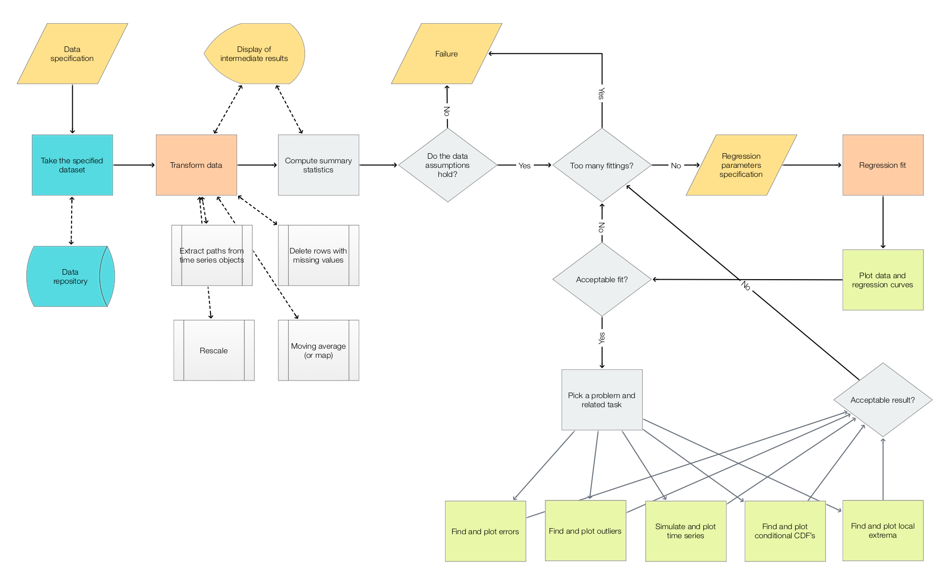
Workflows flowchart
The following flowchart summarizes the workflows that are supported by Regressionizer:
Previous work
Roger Koenker implemented the R package “quantreg”, [RKp1]. Anton Antonov implemented the R package “QRMon-R” for the specification of monadic pipelines for doing QR, [AAp1].
Several Wolfram Language (aka Mathematica) packages are implemented by Anton Antonov, see [AAp1, AAp2, AAf1].
Remark: The paclets at the Wolfram Language Paclet Repository were initially Mathematica packages hosted at GitHub. The Wolfram Function Repository function QuantileRegression, [AAf1] does only B-spline fitting.
Setup
Load the “Regressionizer” and other “standard” packages:
from Regressionizer import *

import numpy as np
import plotly.express as px
import plotly.graph_objects as go
template='plotly'
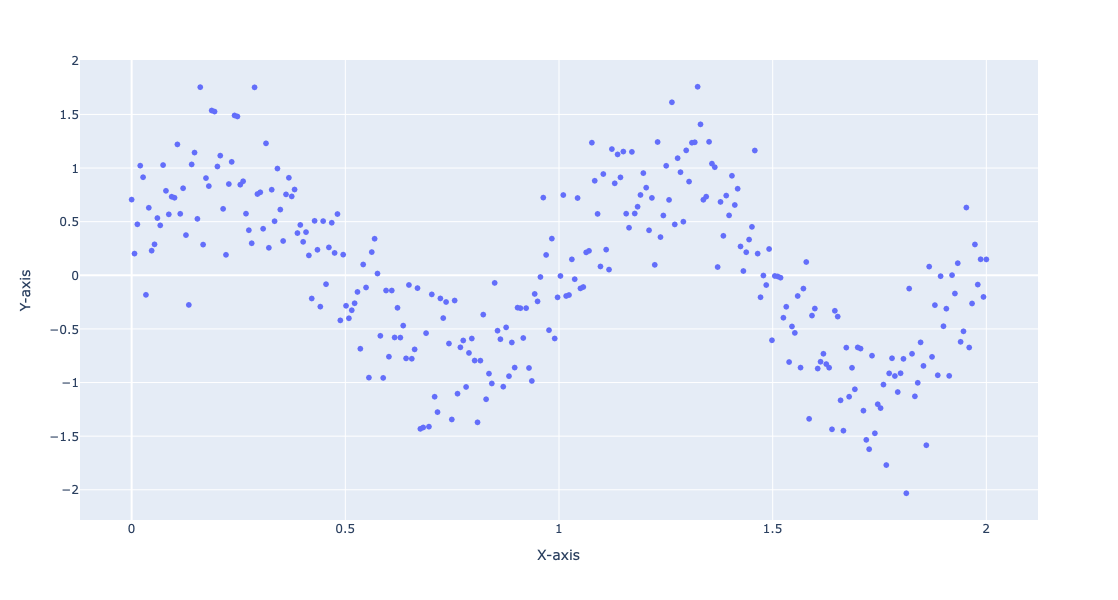
Generate input data
Generate random data:
np.random.seed(0)
x = np.linspace(0, 2, 300)
y = np.sin(2 * np.pi * x) + np.random.normal(0, 0.4, x.shape)
data = np.column_stack((x, y))
Plot the generated data:
fig = px.scatter(x=data[:, 0], y=data[:, 1], labels={'x': 'X-axis', 'y': 'Y-axis'}, template=template, width = 800, height = 600)
fig.show()
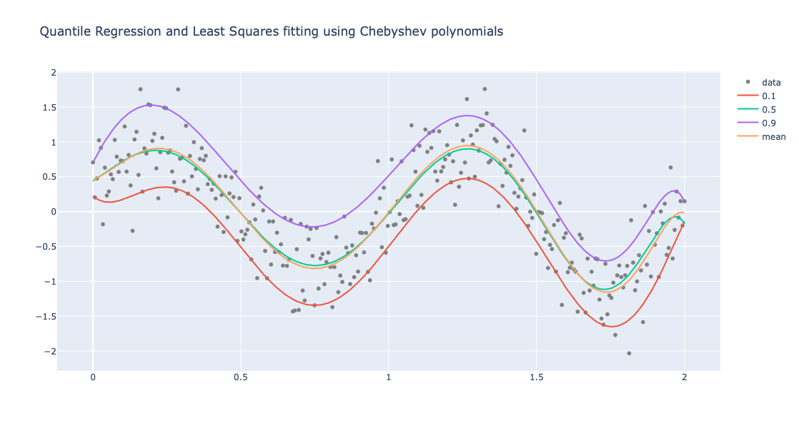
Fit given functions
Define a list of functions:
funcs = [lambda x: 1, lambda x: x, lambda x: np.cos(x), lambda x: np.cos(3 * x), lambda x: np.cos(6 * x)]
def chebyshev_t_polynomials(n):
    if n == 0:
        return lambda x: 1
    elif n == 1:
        return lambda x: x
    else:
        T0 = lambda x: 1
        T1 = lambda x: x
        for i in range(2, n + 1):
            Tn = lambda x, T0=T0, T1=T1: 2 * x * T1(x) - T0(x)
            T0, T1 = T1, Tn
        return Tn

chebyshev_polynomials = [chebyshev_t_polynomials(i) for i in range(10)]
Define regression quantile probabilities:
probs = [0.1, 0.5, 0.9]
Perform Quantile Regression and (non-linear) Least Squares Fit:
obj2 = (
    Regressionizer(data)
    .echo_data_summary()
    .quantile_regression_fit(funcs=chebyshev_polynomials, probs=probs)
    .least_squares_fit(funcs=chebyshev_polynomials)
    .plot(title = "Quantile Regression and Least Squares fitting using Chebyshev polynomials", template=template)
)
Statistic    Regressor | Value
------------ --------------------
min                 0.0 | -2.0324132316043735
25%                 0.5 | -0.6063257640389526
median              1.0 | -0.0042185202753221695
75%                 1.5 | 0.6300535444986601
max                 2.0 | 1.757964402499859
Plot the obtained regression quantilies and least squares fit:
obj2.take_value().show()
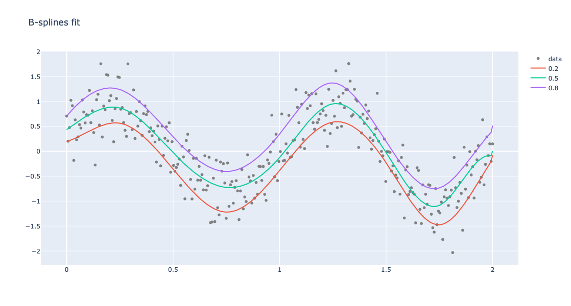
Fit B-splines
Instead of coming-up with basis functions we can use B-spline basis:
obj = Regressionizer(data).quantile_regression(knots=8, probs=[0.2, 0.5, 0.8]).plot(title="B-splines fit", template=template)
Show the obtained plot:
obj.take_value().show()
Here is a dictionary of the found regression quantiles:
obj.take_regression_quantiles()
{0.2: <function QuantileRegression.QuantileRegression._make_combined_function.<locals>.<lambda>(x)>,
 0.5: <function QuantileRegression.QuantileRegression._make_combined_function.<locals>.<lambda>(x)>,
 0.8: <function QuantileRegression.QuantileRegression._make_combined_function.<locals>.<lambda>(x)>}
Weather temperature data
Load weather data:
import pandas as pd

url = "https://raw.githubusercontent.com/antononcube/MathematicaVsR/master/Data/MathematicaVsR-Data-Atlanta-GA-USA-Temperature.csv"
dfTemperature = pd.read_csv(url)
dfTemperature['DateObject'] = pd.to_datetime(dfTemperature['Date'], format='%Y-%m-%d')
dfTemperature = dfTemperature[(dfTemperature['DateObject'].dt.year >= 2020) & (dfTemperature['DateObject'].dt.year <= 2023)]
dfTemperature
| Date | AbsoluteTime | Temperature | DateObject | |
|---|---|---|---|---|
| 2555 | 2020-01-01 | 3786825600 | 7.56 | 2020-01-01 |
| 2556 | 2020-01-02 | 3786912000 | 7.28 | 2020-01-02 |
| 2557 | 2020-01-03 | 3786998400 | 12.28 | 2020-01-03 |
| 2558 | 2020-01-04 | 3787084800 | 12.78 | 2020-01-04 |
| 2559 | 2020-01-05 | 3787171200 | 4.83 | 2020-01-05 |
| … | … | … | … | … |
| 4011 | 2023-12-27 | 3912624000 | 11.67 | 2023-12-27 |
| 4012 | 2023-12-28 | 3912710400 | 7.44 | 2023-12-28 |
| 4013 | 2023-12-29 | 3912796800 | 3.78 | 2023-12-29 |
| 4014 | 2023-12-30 | 3912883200 | 4.83 | 2023-12-30 |
| 4015 | 2023-12-31 | 3912969600 | 1.17 | 2023-12-31 |
1461 rows × 4 columns
Convert to “numpy” array:
temp_data = dfTemperature[['AbsoluteTime', 'Temperature']].to_numpy()
temp_data.shape
(1461, 2)
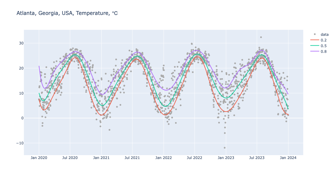
Here is pipeline for Quantile Regression computation and making of a corresponding plot:
obj = (
    Regressionizer(temp_data)
    .echo_data_summary()
    .quantile_regression(knots=20, probs=[0.2, 0.5, 0.8])
    .date_list_plot(title="Atlanta, Georgia, USA, Temperature, ℃", template=template, data_color="darkgray", width = 1200)
)
Statistic    Regressor | Value
------------ --------------------
min          3786825600.0 |     -11.89
25%          3818361600.0 |      10.06
median       3849897600.0 |      16.94
75%          3881433600.0 |      22.56
max          3912969600.0 |      32.39
Show the obtained plot:
obj.take_value().show()
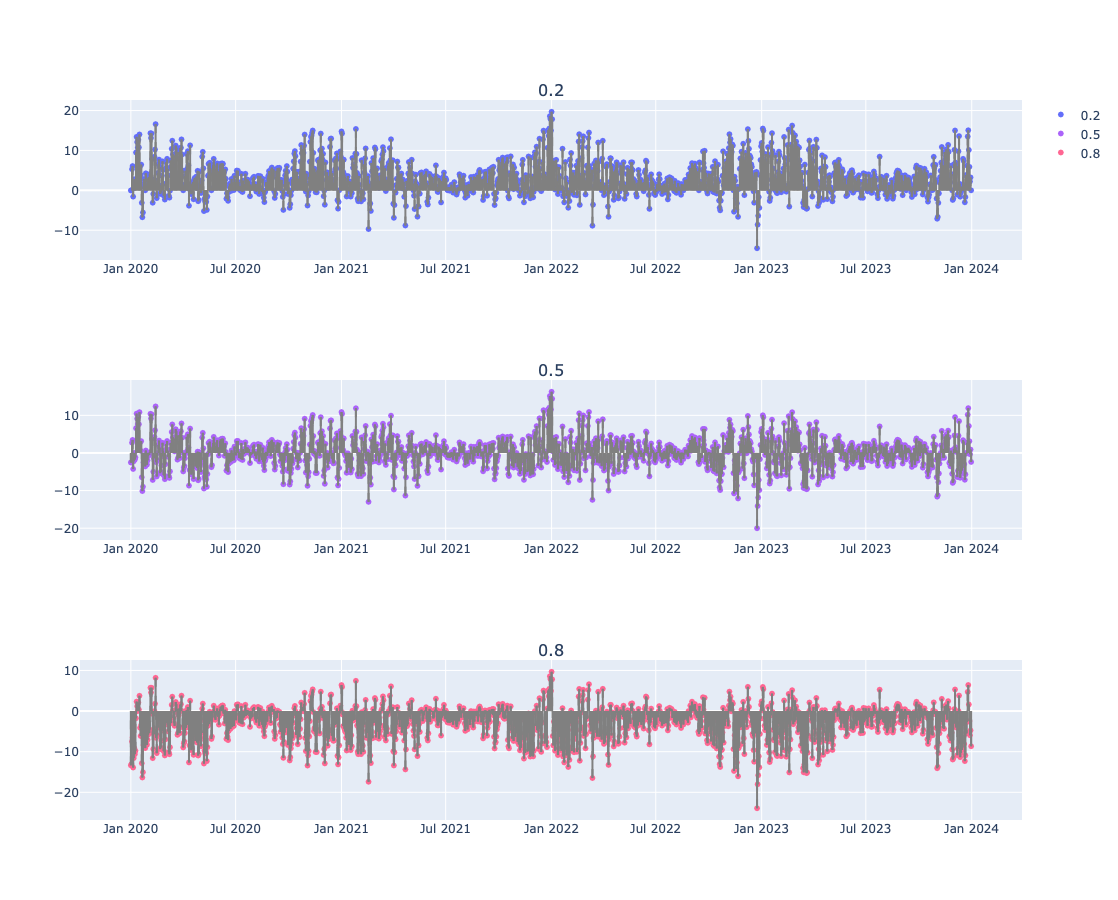
Fitting errors
Errors
Here the absolute fitting errors are computed and the average is for each is computed:
{ k : np.mean(np.array(d)[:,1]) for k, d in obj.errors(relative_errors=False).take_value().items() }
{0.2: 3.331223347420249, 0.5: 0.020191754857989016, 0.8: -3.3960272281557753}
Error plots
Here we give the fitting errors (residuals) for the regression quantiles found and plotted above:
obj.error_plots(relative_errors=False, date_plot=True, template=template, width=1200, height=300).take_value().show()
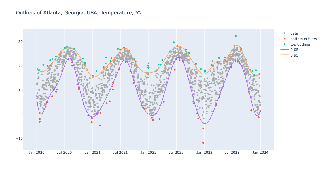
Outliers
One way to find contextual outliers in time series is to find regression quantiles at low- and high enough probabilities, and then select the points “outside” of those curves:
obj = (
    Regressionizer(temp_data)
    .quantile_regression(knots=20, probs=[0.01,  0.99], order=3)
    .outliers()
)

obj.take_value()
{'bottom': [array([ 3.7885536e+09, -3.1100000e+00]),
  array([3.7919232e+09, 3.2800000e+00]),
  array([3.795552e+09, 7.390000e+00]),
  array([3.7977984e+09, 9.2800000e+00]),
  array([3.7982304e+09, 1.0220000e+01]),
  array([3.8068704e+09, 2.0110000e+01]),
  array([3.8097216e+09, 1.2390000e+01]),
  array([ 3.8225088e+09, -4.7200000e+00]),
  array([3.8298528e+09, 1.0220000e+01]),
  array([3.8333952e+09, 1.8720000e+01]),
  array([3.8458368e+09, 3.5000000e+00]),
  array([ 3.8524896e+09, -2.3900000e+00])],
 'top': [array([3.7944288e+09, 2.2390000e+01]),
  array([3.802896e+09, 2.756000e+01]),
  array([3.8040192e+09, 2.7940000e+01]),
  array([3.8129184e+09, 2.3000000e+01]),
  array([3.814128e+09, 2.128000e+01]),
  array([3.820608e+09, 1.778000e+01]),
  array([3.8258784e+09, 2.3500000e+01]),
  array([3.8326176e+09, 2.7060000e+01]),
  array([3.839184e+09, 2.617000e+01]),
  array([3.8420352e+09, 2.2780000e+01]),
  array([3.8641536e+09, 2.9830000e+01]),
  array([3.8727072e+09, 2.5610000e+01]),
  array([3.8816928e+09, 1.8060000e+01])]}
Here we plot the outliers (using a “narrower band” than above):
obj = (
    Regressionizer(temp_data)
    .quantile_regression(knots=20, probs=[0.05,  0.95], order=3)
    .outliers_plot(
        title="Outliers of Atlanta, Georgia, USA, Temperature, ℃",
        data_color="darkgray",
        date_plot=True,
        template=template,
        width = 1200)
)

obj.take_value().show()
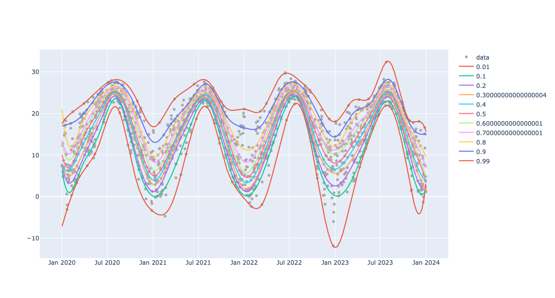
Conditional CDF
Here is a list of probabilities to be used to reconstruct Cumulative Distribution Functions (CDFs):
probs = np.sort(np.concatenate((np.arange(0.1, 1.0, 0.1), [0.01, 0.99])))
probs
array([0.01, 0.1 , 0.2 , 0.3 , 0.4 , 0.5 , 0.6 , 0.7 , 0.8 , 0.9 , 0.99])
Here we find the regression quantiles for those probabilities:
obj=(
    Regressionizer(temp_data)
    .quantile_regression(knots=20,probs=probs)
    .date_list_plot(template=template, data_color="darkgray", width=1200)
    )
Here we show the plot obtained above:
obj.take_value().show()
Get CDF function
Here we take a date in ISO format and convert to number of seconds since 1900-01-01:
from datetime import datetime

iso_date = "2022-01-01"
date_object = datetime.fromisoformat(iso_date)
epoch = datetime(1900, 1, 1)

focusPoint = int((date_object - epoch).total_seconds())
print(focusPoint)
3849984000
Here the conditional CDF at that date is computed:
aCDFs = obj.conditional_cdf(focusPoint).take_value()
aCDFs
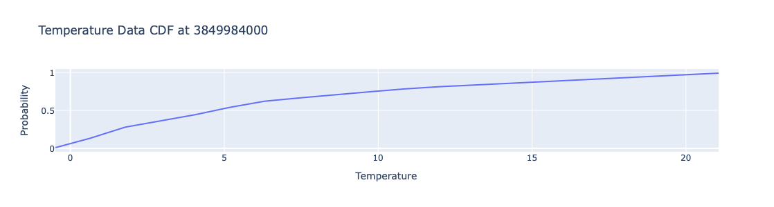
{3849984000: <scipy.interpolate._interpolate.interp1d at 0x135c2c460>}
Plot the obtained CDF function:
xs = np.linspace(obj.take_regression_quantiles()[0.01](focusPoint), obj.take_regression_quantiles()[0.99](focusPoint), 20)
cdf_values = [aCDFs[focusPoint](x) for x in xs]

fig = go.Figure(data=[go.Scatter(x=xs, y=cdf_values, mode='lines')])
# Update layout
fig.update_layout(
    title='Temperature Data CDF at ' + str(focusPoint),
    xaxis_title='Temperature',
    yaxis_title='Probability',
    template=template,
    legend=dict(title='Legend'),
    height=300,
    width=800
)
fig.show()
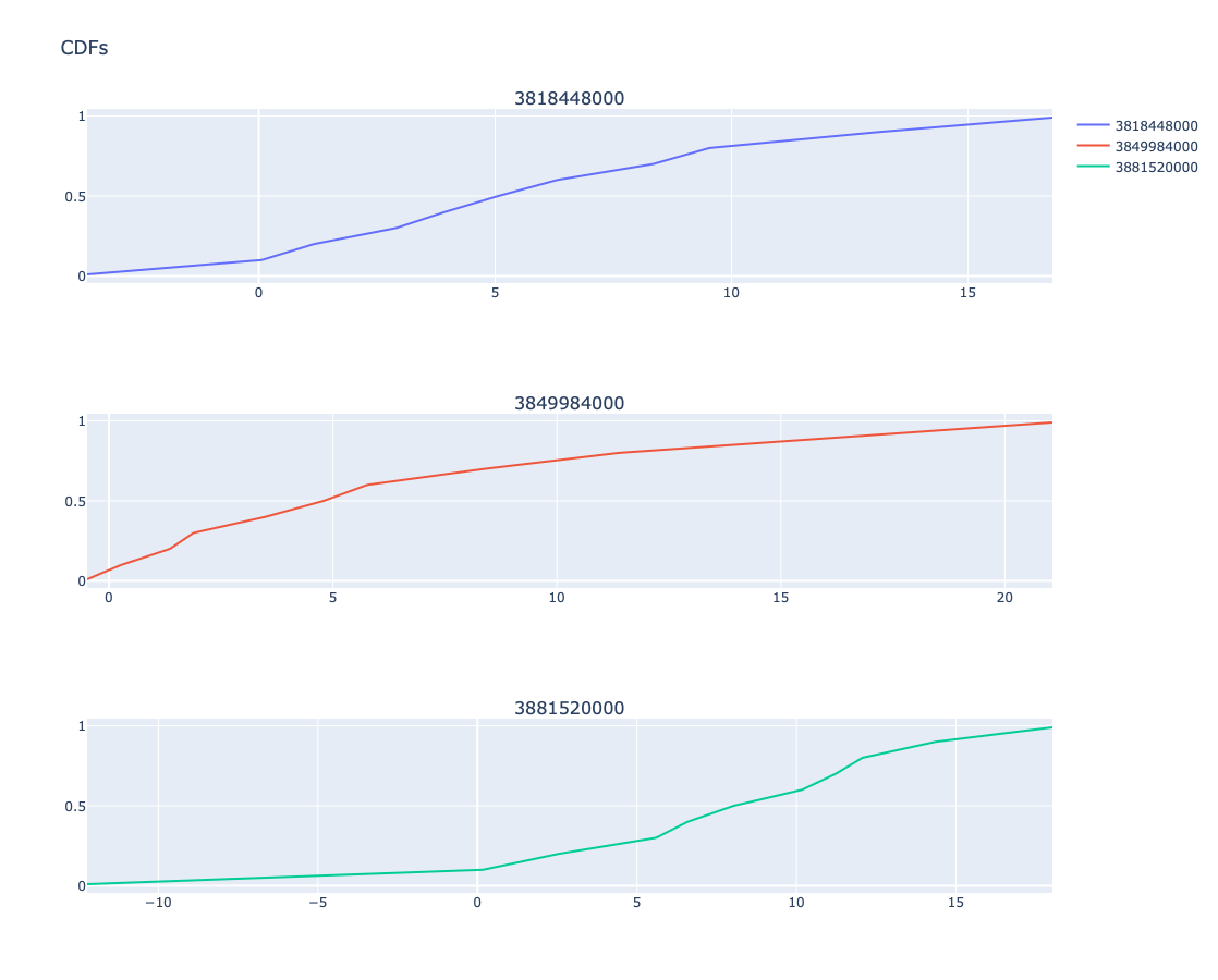
Plot multiple CDFs
Here are few dates converted into number of seconds since 1990-01-01:
pointsForCDFs = [focusPoint + i * 365 * 24 * 3600 for i in range(-1,2)]
pointsForCDFs
[3818448000, 3849984000, 3881520000]
Here are the plots of CDF at those dates:
obj.conditional_cdf_plot(pointsForCDFs, title = 'CDFs', template=template).take_value().show()
References
Articles, books
[RK1] Roger Koenker, Quantile Regression, Cambridge University Press, 2005.
[RK2] Roger Koenker, “Quantile Regression in R: a vignette”, (2006), CRAN.
[AA1] Anton Antonov, “A monad for Quantile Regression workflows”, (2018), MathematicaForPrediction at GitHub.
Packages, paclets
[AAp1] Anton Antonov, Quantile Regression Python package, (2024), GitHub/antononcube.
[AAp2] Anton Antonov, QRMon-R, (2019), GitHub/antononcube.
[AAp3] Anton Antonov, Quantile Regression WL paclet, (2014-2023), GitHub/antononcube.
[AAp4] Anton Antonov, Monadic Quantile Regression WL paclet, (2018-2024), GitHub/antononcube.
[AAf1] Anton Antonov, QuantileRegression, (2019), Wolfram Function Repository.
[RKp1] Roger Koenker, quantreg, CRAN.
Repositories
[AAr1] Anton Antonov, DSL::English::QuantileRegressionWorkflows in Raku, (2020), GitHub/antononcube.
Videos
[AAv1] Anton Antonov, “Boston useR! QuantileRegression Workflows 2019-04-18”, (2019), Anton Antonov at YouTube.
[AAv2] Anton Antonov, “useR! 2020: How to simplify Machine Learning workflows specifications”, (2020), R Consortium at YouTube.
]]>