In today’s post, the code in question is a python file containing quite a few functions from R’s PerformanceAnalytics library outside of Return.portfolio (or Return_portfolio, as it may be in Python, because the . operator is reserved in Python…ugh).

So, here is the “library” of new functions, for now called edhec_perfa.py, as a nod to Vijay Vaidyanathan’s Coursera course(s).

Here’s the link to the latest github file.

Now, while a lot of the functions should be pretty straightforward (annualized return, VaR, CVaR, tracking error/annualized tracking error, etc.), two functions that I think are particularly interesting that I ported over from R with the help of chatGPT (seriously, when prompted correctly, an LLM is quite helpful in translating from one programming language to another, provided the programmer has enough background in both languages to do various debugging) are charts_PerformanceSummary, which does exactly what you might think it does from seeing me use the R function here on the blog, and table_Drawdowns, which gives the highest N drawdowns by depth.

Here’s a quick little Python demo (once you import my file from the github):

import yfinance as yf
import pandas as pd
import numpy as np

symbol = "SPY"
start_date = "1990-01-01"
end_date = pd.Timestamp.today().strftime("%Y-%m-%d")
df_list = []

data = pd.DataFrame(yf.download(symbol, start=start_date, end=end_date))
data = data["Adj Close"]
data.name = symbol
data = pd.DataFrame(data)

returns = Return_calculate(data)

charts_PerformanceSummary(returns)
table_Drawdowns(returns)

This results in the following:

And the following table:

The NaT in the “To” column means that the drawdown is current, as does the NaN in the Recovery–they’re basically Python’s equivalent of NAs, though NaT means an NA on *time*, while an NaN means an NA on a numerical value. So that’s interesting in that Python gives you a little more information regarding your column data types, which is kind of interesting.

Another function included in this library, as a utility function is the infer_trading_periods function. Simply, plug in a time series, and it will tell you the periodicity of the data. Pandas was supposed to have a function that did this, but due to differences in frequency of daily data caused by weekends and holidays, this actually doesn’t work on financial data, so I worked with chatGPT to write a new function that works more generally. R’s checkData function is also in this library (translated over to Python), but I’m not quite sure where it was intended to be used, but left it in for those that want it.

So, for those interested, just feel free to read through some of the functions, and use whichever ones you find applicable to your workflow. That said, if you *do* wind up using it, please let me know, since there’s more value I can add.

Lastly, I’m currently in the job market *and* have a volatility trading signal subscription available to offer for those interested. You can email me at [email protected] or find me on my LinkedIn profile here.

Thanks for reading.

Now, here’s the link to my github for the code for Return.portfolio in Python–or, rather, since the dot operator has a special use in Python, the Return_portfolio function.

But for the record, here’s the Python code, including the endpoints function.

def endpoints(df, on = "M", offset = 0):
    """
    Returns index of endpoints of a time series analogous to R's endpoints
    function.
    Takes in:
        df -- a dataframe/series with a date index
         
        on -- a string specifying frequency of endpoints
         
        (E.G. "M" for months, "Q" for quarters, and so on)
         
        offset -- to offset by a specified index on the original data
        (E.G. if the data is daily resolution, offset of 1 offsets by a day)
        This is to allow for timing luck analysis. Thank Corey Hoffstein.
    """
     
    # to allow for familiarity with R
    # "months" becomes "M" for resampling
    if len(on) > 3:
        on = on[0].capitalize()
     
    # get index dates of formal endpoints
    ep_dates = pd.Series(df.index, index = df.index).resample(on).max()
     
    # get the integer indices of dates that are the endpoints
    date_idx = np.where(df.index.isin(ep_dates))
     
    # append last day to match R's endpoints function
    # remember, Python is indexed at 0, not 1
    #date_idx = np.insert(date_idx, 0, 0)
    date_idx = np.append(date_idx, df.shape[0]-1)
    if offset != 0:
        date_idx = date_idx + offset
        date_idx[date_idx < 0] = 0
        date_idx[date_idx > df.shape[0]-1] = df.shape[0]-1
    out = np.unique(date_idx)
    return out  

def compute_weights_and_returns(subset_returns, weights):
  rep_weights = np.tile(weights, (len(subset_returns), 1))
  cum_subset_weights = np.cumprod(1 + subset_returns, axis=0) * rep_weights
  EOP_Weight = cum_subset_weights / np.sum(cum_subset_weights, axis=1).to_numpy()[:, np.newaxis]
  cum_subset_weights_bop = cum_subset_weights / (1 + subset_returns)
  BOP_Weight = cum_subset_weights_bop / np.sum(cum_subset_weights_bop, axis=1).to_numpy()[:, np.newaxis]
  portf_returns_subset = pd.DataFrame(np.sum(subset_returns.values * BOP_Weight, axis=1), 
                                        index=subset_returns.index, columns=['Portfolio.Returns'])
  return [portf_returns_subset, BOP_Weight, EOP_Weight]


# Return.portfolio.geometric from R
def Return_portfolio(R, weights=None, verbose=True, rebalance_on='months'):
  """

    Parameters
    ----------
    R : a pandas series of asset returns
    weights : a vector or pandas series of asset weights.
    verbose : a boolean specifying a verbose output containing:
        portfolio returns,
        beginning of period weights and values, end of period weights and values,
        asset contribution to returns, and two-way turnover calculation
    rebalance_on : a string specifying rebalancing frequency if weights are passed in as a vector.

    Raises
    ------
    ValueError
        Number of asset weights must be equal to the number of assets.

    Returns
    -------
    TYPE
        See verbose parameter for True value, otherwise just portfolio returns.

    """
  
  # make sure original object isn't overridden
  R = R.copy()
  weights = weights.copy()
  
  # impute NAs in returns
  if R.isna().sum().sum() > 0:
    R.fillna(0, inplace=True)
    wn.warn("NAs detected in returns. Imputing with zeroes.")
    
    # if no weights provided, create equal weight vector
  if weights is None:
    weights = np.repeat(1/R.shape[1], R.shape[1])
    wn.warn("Weights not provided, assuming equal weight for rebalancing periods.")
    
    # if weights aren't passed in as a data frame (they're probably a list)
    # turn them into a 1 x num_assets data frame
  if type(weights) != pd.DataFrame:
    weights = pd.DataFrame(weights)
    weights = weights.transpose()
    
    # error checking for same number of weights as assets
  if weights.shape[1] != R.shape[1]:
        raise ValueError("Number of weights is unequal to number of assets. Correct this.")
    
    
  # if there's a row vector of weights, create a data frame with  the desired 
  # rebalancing schedule --  also add in the very first date into the schedule
  if weights.shape[0] == 1:
        if rebalance_on is not None:
            ep = endpoints(R, on = rebalance_on)
            first_weights = pd.DataFrame(np.array(weights), index=[R.index[0]], columns=R.columns)
            weights = pd.concat([first_weights, pd.DataFrame(np.tile(weights, 
                        (len(ep), 1)), index=R.index[ep], columns=R.columns)], axis=0)
            #weights = pd.DataFrame(np.tile(weights, (len(ep), 1)), 
            #                       index = ep.index, columns = R.columns)
            weights.index.name = R.index.name
        else:
            weights = pd.DataFrame(weights, index=[R.index[0]], columns=R.columns)
    
  original_weight_dim = weights.shape[1] # save this for computing two-way turnover

    
  if weights.isna().sum().sum() > 0:
    weights.fillna(0, inplace=True)
    wn.warn("NAs detected in weights. Imputing with zeroes.")
    
  residual_weights = 1 - weights.sum(axis=1)
  if abs(residual_weights).sum() != 0:
    print("One or more periods do not have investment equal to 1. Creating residual weights.")
    weights["Residual"] = residual_weights
    R["Residual"] = 0
    
  if weights.shape[0] != 1:
    portf_returns, bop_weights, eop_weights = [], [], []
    for i in range(weights.shape[0]-1):
      subset = R.loc[(R.index >= weights.index[i]) & (R.index <= weights.index[i+1])]
      if i >= 1: # first period include all data
                # otherwise, final period of previous period is included, so drop it
        subset = subset.iloc[1:]
      subset_out = compute_weights_and_returns(subset, weights.iloc[i,:])
      subset_out[0].columns = ["Portfolio.Returns"]
      portf_returns.append(subset_out[0])
      bop_weights.append(subset_out[1])
      eop_weights.append(subset_out[2])
    portf_returns = pd.concat(portf_returns, axis=0)
    bop_weights = pd.concat(bop_weights, axis=0)
    eop_weights = pd.concat(eop_weights, axis=0)
  else: # only one weight allocation at the beginning and just drift the portfolio
    out = compute_weights_and_returns(R, weights)
    portf_returns = out[0]; portf_returns.columns = ['Portfolio.Returns']
    bop_weights = out[1]
    eop_weights = out[2]
    
    
  pct_contribution = R * bop_weights
  cum_returns = (1 + portf_returns).cumprod()
  eop_value = eop_weights * pd.DataFrame(np.tile(cum_returns, (1, eop_weights.shape[1])), 
                                        index=eop_weights.index, columns=eop_weights.columns)
  bop_value = bop_weights * pd.DataFrame(np.tile(cum_returns/(1+portf_returns), (1, bop_weights.shape[1])), 
                                        index=bop_weights.index, columns=bop_weights.columns)

  turnover = (np.abs(bop_weights.iloc[:, :(original_weight_dim-1)] - eop_weights.iloc[:, :(original_weight_dim-1)].shift(1))).sum(axis=1).dropna()
  turnover = pd.DataFrame(turnover, index=eop_weights.index[1:], columns=['Two-way turnover'])

  out = [portf_returns, pct_contribution, bop_weights, eop_weights, bop_value, eop_value, turnover]
  out = {k: v for k, v in zip(['returns', 'contribution', 'BOP.Weight', 'EOP.Weight', 'BOP.Value', 'EOP.Value', 'Two.Way.Turnover'], out)}
  if verbose:
        return out
  else:
        return portf_returns

Rather than go into it line by line, those interested can read the code, but ultimately, a lot of it is basically seeing if the weights were passed in as a data frame of individually customized weights (E.G. on January, my weights were such and such, and on February, they shifted to some other such and such), or if the weights were passed in as a vector, or Python list, if someone just wants to rebalance a portfolio (E.G. a classic buy-and-hold 60/40), and if some portfolio weights don’t add up to 1. Essentially, a fair bit of bookkeeping. (Speaking of, I’m not sure what happened to the programming language customization block here on wordpress, so, I sincerely encourage readers to check my github for this code).

Now, here’s the interesting part which motivated this post:

I didn’t write most of this code in Python. Or rather, not initially.

I wrote it in R, first, to understand it, with R’s vectorization, where I’m a bit more comfortable. (As an aside, as far as languages for quantitative finance go, I think R has the much more advanced buy-side libraries such as PortfolioAnalytics or Quantstrat compared to Python, as they were written by high-level industry practitioners, whereas Python’s finance ecosystem seems to be…fairly threadbare, consisting of various islands of libraries that don’t really play together all that well.)

Here’s the R code that I did to rewrite Peter Carl’s Return.portfolio.geometric (the underlying function that runs Return.portfolio that I’ve used all these years):

compute_weights_and_returns <- function(subset, weights) {
  rep_weights <- matrix(nrow=nrow(subset), ncol = ncol(subset), weights, byrow = TRUE)
  cum_subset_weights <- cumprod(1+subset) * rep_weights
  EOP.Weight <- cum_subset_weights/rowSums(cum_subset_weights)
  cum_subset_weights_bop <- cum_subset_weights/(1+subset)
  BOP.Weight <- cum_subset_weights_bop/rowSums(cum_subset_weights_bop)
  portf_returns_subset <- xts(rowSums(subset * BOP.Weight), order.by=index(subset))
  return(list(portf_returns_subset, BOP.Weight, EOP.Weight))
}

Return.portfolio.geometric.ilya <- function(R, weights, verbose = TRUE, rebalance_on = 'months') {
  
  if(sum(is.na(R)) > 0) {
    R[is.na(R)] <- 0
    warning("NAs detected in returns. Imputing with zeroes.")
  }
  
  if(missing(weights)) {
    weights <- rep(1/ncol(R), ncol(R))
    warning("Weights not provided, assuming equal weight for rebalancing periods.")
  }
  
  # if weights passed in as vector
  if(is.null(dim(weights))) {
    if(!is.null(rebalance_on)) {
      ep <- endpoints(R)
      first_weights <- xts(t(matrix(weights)), order.by=index(R)[1])
      weights <- rbind(first_weights,
                           xts(matrix(nrow=length(index(R)[ep]), 
                                      ncol = length(weights), weights, byrow=TRUE),
                             order.by = index(R)[ep]))
      # get the first day of all the weights, make sure it's unique
      # weights <- weights[!duplicated(index(weights)),]
    } else {
      weights <- xts(t(matrix(weights)), order.by=index(R)[1])
    }
    colnames(weights) <- colnames(R)
  } 
  
  original_weight_dim <- ncol(weights) # save this for computing two-way turnover
  
  if(original_weight_dim != ncol(R)) {
    stop("Number of weights is unequal to number of assets. Correct this.")
  }
  
  if(sum(is.na(weights)) > 0) {
    weights[is.na(weights)] <- 0
    warning("NAs detected in weights. Imputing with zeroes.")
  }
  
  residual_weights <- 1-rowSums(weights)
  if(sum(abs(residual_weights)) != 0) {
    warning("One or more periods do not have investment equal to 1. Creating residual weights.")
    weights$Residual <-  residual_weights
    R$Residual <- 0
  }
  if(nrow(weights) != 1) {
    portf_returns <- bop_weights <- eop_weights <- list()
    for(i in 1:(nrow(weights)-1)) {
      subset <- R[paste((index(weights)[i]),index(weights)[i+1], sep = "::"),]
      if(i >= 2) { # first period include all data
        # otherwise, final period of previous period is included, so drop it
        subset <- subset[-1,]
      }
      subset_out <- compute_weights_and_returns(subset, weights[i,])
      colnames(subset_out[[1]]) <- "Portfolio.Returns"
      portf_returns[[i]] <- subset_out[[1]]
      bop_weights[[i]] <- subset_out[[2]]
      eop_weights[[i]] <- subset_out[[3]]
    }
    portf_returns <- do.call(rbind, portf_returns)
    bop_weights <- do.call(rbind, bop_weights)
    eop_weights <- do.call(rbind, eop_weights)
  } else { # only one weight allocation at the beginning and just drift the portfolio
    out <- compute_weights_and_returns(R, weights)
    portf_returns <- out[[1]]; colnames(portf_returns) <- "Portfolio.Returns"
    bop_weights <- out[[2]]
    eop_weights <- out[[3]]
  }
  pct_contribution <- R * bop_weights
  cum_returns <- cumprod(1+portf_returns)
  eop_value <- eop_weights * matrix(nrow=nrow(eop_weights), ncol = ncol(eop_weights), 
                                    cum_returns, byrow= FALSE) 
  bop_value <- bop_weights * matrix(nrow=nrow(bop_weights), ncol = ncol(bop_weights),
                                    cum_returns/(1+portf_returns), byrow = FALSE)
  
  # add turnover computation because that's what this whole exercise is about
  turnover <- na.omit(xts(rowSums(abs(bop_weights[,1:original_weight_dim] - 
                                        lag(eop_weights[,1:original_weight_dim]))), 
                          order.by = index(eop_weights)))
  
  colnames(turnover) <- "Two-way turnover"
  
  out <- list(portf_returns, pct_contribution, bop_weights, 
              eop_weights, bop_value, eop_value, turnover)
  names(out) <- c("returns", "contribution", "BOP.Weight", 
                  "EOP.Weight", "BOP.Value", "EOP.Value", "Two.Way.Turnover")
  if(verbose) {
    return(out)
  } else {
    return(portf_returns)
  }
}

Now, how did I go from the above to the code at the beginning of this post?

ChatGPT4.

That is, I translated my R code into Python code using ChatGPT4 by simply having it translate, block by block, my R code into Python.

Now, was it perfect? No, actually. I had to run the code block by block, and do a little bit of debugging here and there–including adding the functionality for the Return_portfolio function to make deep copies of the returns and weights, instead of modifying the original data structure passed into the function, since Python by default is a pass by reference language, not pass by value (ugh). However, this sort of “Rosetta Stone” functionality inherent in ChatGPT4 is occasionally useful.

Now, when I first tried prompting chatGPT4 to just translate R’s functions, without guiding it step by step, it was a total disaster. Contrary to popular belief, ChatGPT4 is *not* some all-powerful, all-perfect, all-knowing, and all-wise (as the late, great, George Carlin once said) system. But occasionally, it can be useful.

Furthermore, as someone that’s used AI to try my hand at image generation, I also consider those systems (such as StableDiffusion, or Leonardo.AI) to be…somewhat impressive, if in their infancy right now (it gets much more difficult to have multiple subjects interact on one image–I.E. if you want to describe one person in an image, that’s one thing, but if you want to describe two, it isn’t like you can make an image of one–say, save it with a name, such as Alice.jpeg, make an image of a second, save it to another name, such as Bob.jpeg, and then say “Alice being hugged by Bob”). Of course, I’ve definitely been aware about the copyright hubbub brewing over the image generating AI space, but as someone that’s given away plenty of code over the past 8 or so years, including code that has been augmented to run $87 million at a $1B AUM fund, I’m pretty squarely on the open source side, even if seeing my code being responsible for running more than $100 million in AUM, and not getting paid residuals on the management fees, has discouraged me from continuing to share strategy research (I was always of the opinion that anything I shared using freely available Yahoo data was something that large investment houses had already passed over and run a more sophisticated variant of–apparently, this isn’t the case, so giving away strategy code for free nowadays seems like a very suspect thing to do).

In any case, using image-generating AI has allowed me to make artwork the likes of which I never dreamed of creating before, so I’m of the opinion that a few people taking the side of IP hoarding corporations (such as big pharma hoarding insulin patents, or Disney continuing to milk Mickey Mouse) can go kick rocks, and that IP law has long overreached. That said, I already have StableDiffusion running on my machine, coupled with some more sophisticated models built on top of it (Dreamshaper v5, Deliberate v2, etc.), and still have a lot to learn about it–though I’ll probably need a more powerful machine than a gaming laptop to really crank images out.

Now, my thoughts on AI? So far, I don’t think that AI alone is going to pull a South Park and DERK YERRR JERBZ. At least if you’re a skilled professional.

Not alone, anyway. And for what it’s worth, as a quantitative research analyst, I found that I’d fire ChatGPT4 within a few hours, owing to the artifact of AI hallucinations. As the phrase goes, trust *but verify*. I think we’re still far, far away from ChatGPT4 being able to read a strategy paper on Quantpedia, replicating it in R or Python, running the code, and replicating the results. For that matter, I think that any strategy paper submission or blog post is incomplete without data and code, for immediate replication, ready to go. It’s the 21st century. Github or git out. A minimum reproducible example (MRE) as a demo of the concept (even a toy one), in my opinion, is vastly more useful than 25 pages of mathematical derivation. Though that’s just me speaking given my background of hands-on engineering and actually *doing things* rather than merely theorizing about them.

Okay, so…this post seems to have gotten long in the tooth. In other news, I’m in the job market, currently, and as I’ve shown, I have a fairly solid command of Python, having several years of off and on experience with it. And I’m also wondering if a written blog is the best way to actually communicate so many of my findings, or if YouTube is the way to go (though I don’t know much about editing videos).

So…yeah. Follow if you like the post, and most importantly:

Try to lose money…less than I do.

Thanks for reading.

My LinkedIn.

So, first off, with those not familiar, there was an article about this proposed ETF published about a month ago. You can read it here. The long story short is that this ETF is created by one Stuart Barton, who also manages InvestInVol. From conversations with Stuart, I can vouch for the fact that he strikes me as very knowledgeable in the vol space, and, if I recall correctly, was one of the individuals that worked on the original VXX ETF at Barclay’s. So when it comes to creating a newer, safer vehicle for trading short-term short vol, I’d venture to think he’s about as good as any.

In any case, here’s a link to my Python notebook, ahead of time, which I will now discuss here, on this post.

So first off, we’ll start by getting the data, and in case anyone forgot what XIV did in 2018, here’s a couple of plots.

import numpy as np
import pandas as pd
import scipy.stats as stats
import matplotlib.pyplot as plt
from pandas_datareader import data
import datetime as dt
from datetime import datetime

# get XIV from a public dropbox -- XIV had a termination event Feb. 5 2018, so this is archived data.

xiv = pd.read_csv("https://dl.dropboxusercontent.com/s/jk6der1s5lxtcfy/XIVlong.TXT", parse_dates=True, index_col=0)

# get SVXY data from Yahoo finance
svxy = data.DataReader('SVXY', 'yahoo', '2016-01-01')
#yahoo_xiv = data.DataReader('XIV', 'yahoo', '1990-01-01')

# yahoo no longer carries XIV because the instrument blew up, need to find it from historical sources
xiv_returns = xiv['Close'].pct_change()
svxy_returns = svxy['Close'].pct_change()

xiv['Close'].plot(figsize=(20,10))
plt.show()
xiv['2016':'2018']['Close'].plot(figsize=(20,10))

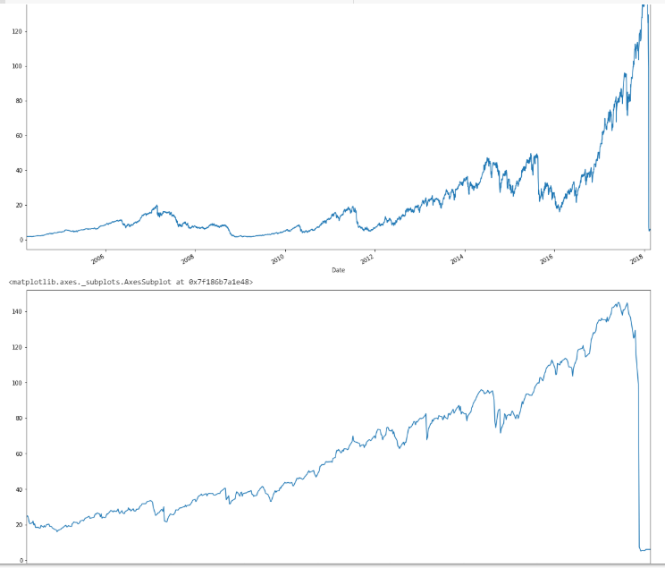
Yes, for those new to the blog, that event actually happened, and in the span of 20 minutes (my trading system got to the sideline about a week before, and even had I been in–which I wasn’t–I would have been in ZIV), during which time XIV blew up in after-hours trading. Immediately following, SVXY (which survived), deleveraged to a 50% exposure.

In any case, here’s the code to get SVIX data from my dropbox, essentially to the end of 2019, after I manually did some work on it because the CBOE has it in a messy format, and then to combine it with the combined XIV + SVXY returns data. (For the record, the SVIX hypothetical performance can be found here on the CBOE website)

# get formatted SVIX data from my dropbox (CBOE has it in a mess)

svix = pd.read_csv("https://www.dropbox.com/s/u8qiz7rh3rl7klw/SHORTVOL_Data.csv?raw=1", header = 0, parse_dates = True, index_col = 0)
svix.columns = ["Open", "High", "Low", "Close"]
svix_rets = svix['Close'].pct_change()

# put data set together

xiv_svxy = pd.concat([xiv_returns[:'2018-02-07'],svxy_returns['2018-02-08':]], axis = 0)
xiv_svxy_svix = pd.concat([xiv_svxy, svix_rets], axis = 1).dropna()
xiv_svxy_svix.tail()

final_data = xiv_svxy_svix
final_data.columns = ["XIV_SVXY", "SVIX"]

One thing that can be done right off the bat (which is a formality) is check if the distributions of XIV+SVXY or SVIX are normal in nature.

print(stats.describe(final_data['XIV_SVXY']))
print(stats.describe(final_data['SVIX']))
print(stats.describe(np.random.normal(size=10000)))

Which gives the following output:

DescribeResult(nobs=3527, minmax=(-0.9257575757575758, 0.1635036496350366), mean=0.0011627123490346562, variance=0.0015918321320673623, skewness=-4.325358554250933, kurtosis=85.06927230848028)
DescribeResult(nobs=3527, minmax=(-0.3011955533480766, 0.16095949898733686), mean=0.0015948970447533636, variance=0.0015014216189676208, skewness=-1.0811171524703087, kurtosis=4.453114992142524)
DescribeResult(nobs=10000, minmax=(-4.024990382591559, 4.017237262611489), mean=-0.012317646021121993, variance=0.9959681097965573, skewness=0.00367629631713188, kurtosis=0.0702696931810931)

Essentially, both of them are very non-normal (obviously), so any sort of statistical comparison using t-tests isn’t really valid. That basically leaves the Kruskal-Wallis test and Wilcoxon signed rank test to see if two data sets are different. From a conceptual level, the idea is fairly straightforward: the Kruskal-Wallis test is analogous to a two-sample independent t-test to see if one group differs from another, while the Wilcoxon signed rank test is analogous to a t-test of differences, except both use ranks of the observations rather than the actual values themselves.

Here’s the code for that:

stats.kruskal(final_data['SVIX'], final_data['XIV_SVXY'])
stats.wilcoxon(final_data['SVIX'], final_data['XIV_SVXY'])

With the output:

KruskalResult(statistic=0.8613306385456933, pvalue=0.3533665896055551)
WilcoxonResult(statistic=2947901.0, pvalue=0.0070668195307847575)

Essentially, when seen as two completely independent instruments, there isn’t enough statistical evidence to reject the idea that SVIX has no difference in terms of the ranks of its returns compared to XIV + SVXY, which would make a lot of sense, considering that for both, Feb. 5, 2018 was their worst day, and there wasn’t much of a difference between the two instruments prior to Feb. 5. In contrast, when considering the two instruments from the perspective of SVIX becoming the trading vehicle for what XIV used to be, and then comparing the differences against a 50% leveraged SVXY, then SVIX is the better instrument with differences that are statistically significant at the 1% level.

Basically, SVIX accomplishes its purpose of being an improved take on XIV/SVXY, because it was designed to be just that, with statistical evidence of exactly this.

One other interesting question to ask is when exactly did the differences in the Wilcoxon signed rank test start appearing? After all, SVIX is designed to have been identical to XIV prior to the crash and SVXY’s deleveraging. For this, we can use the endpoints function for Python I wrote in the last post.

# endpoints function

def endpoints(df, on = "M", offset = 0):
    """
    Returns index of endpoints of a time series analogous to R's endpoints
    function. 
    Takes in: 
        df -- a dataframe/series with a date index
         
        on -- a string specifying frequency of endpoints
         
        (E.G. "M" for months, "Q" for quarters, and so on)
         
        offset -- to offset by a specified index on the original data
        (E.G. if the data is daily resolution, offset of 1 offsets by a day)
        This is to allow for timing luck analysis. Thank Corey Hoffstein.
    """
     
    # to allow for familiarity with R
    # "months" becomes "M" for resampling
    if len(on) > 3:
        on = on[0].capitalize()
     
    # get index dates of formal endpoints
    ep_dates = pd.Series(df.index, index = df.index).resample(on).max()
     
    # get the integer indices of dates that are the endpoints
    date_idx = np.where(df.index.isin(ep_dates))
     
    # append zero and last day to match R's endpoints function
    # remember, Python is indexed at 0, not 1
    date_idx = np.insert(date_idx, 0, 0)
    date_idx = np.append(date_idx, df.shape[0]-1)
    if offset != 0:
        date_idx = date_idx + offset
        date_idx[date_idx < 0] = 0
        date_idx[date_idx > df.shape[0]-1] = df.shape[0]-1
    out = np.unique(date_idx)
    return out   

ep = endpoints(final_data)

dates = []
pvals = []
for i in range(0, (len(ep)-12)):
  data_subset = final_data.iloc[(ep[i]+1):ep[i+12]]
  pval = stats.wilcoxon(data_subset['SVIX'], data_subset['XIV_SVXY'])[1]
  date = data_subset.index[-1]
  dates.append(date)
  pvals.append(pval)
wilcoxTS = pd.Series(pvals, index = dates)
wilcoxTS.plot(figsize=(20,10))

wilcoxTS.tail(30)

The last 30 points in this monthly time series looks like this:

2017-11-29    0.951521
2017-12-28    0.890546
2018-01-30    0.721118
2018-02-27    0.561795
2018-03-28    0.464851
2018-04-27    0.900470
2018-05-30    0.595646
2018-06-28    0.405771
2018-07-30    0.228674
2018-08-30    0.132506
2018-09-27    0.085125
2018-10-30    0.249457
2018-11-29    0.230020
2018-12-28    0.522734
2019-01-30    0.224727
2019-02-27    0.055854
2019-03-28    0.034665
2019-04-29    0.019178
2019-05-30    0.065563
2019-06-27    0.071348
2019-07-30    0.056757
2019-08-29    0.129120
2019-09-27    0.148046
2019-10-30    0.014340
2019-11-27    0.006139
2019-12-26    0.000558
dtype: float64

And the corresponding chart looks like this:

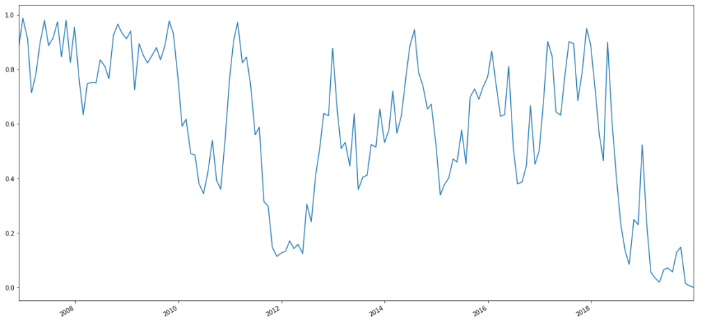
Essentially, about six months after Feb. 5, 2018–I.E. about six months after SVXY deleveraged, we see the p-value for yearly rolling Wilcoxon signed rank tests (measured monthly) plummet and stay there.

So, the long story short is: once SVIX starts to trade, it should be the way to place short-vol, near-curve bets, as opposed to the 50% leveraged SVXY that traders must avail themselves with currently (or short VXX, with all of the mechanical and transaction risks present in that regard).

That said, from having tested SVIX with my own volatility trading strategy (which those interested can subscribe to, though in fair disclosure, this should be a strategy that diversifies a portfolio, and it’s a trend follower that was backtested in a world without Orange Twitler creating price jumps every month), the performance improves from backtesting with the 50% leveraged SVXY, but as I *dodged* Feb. 5, 2018, the results are better, but the risk is amplified as well, because there wasn’t really a protracted sideways market the likes of which we’ve seen the past couple of years for a long while.

In any case, thanks for reading.

NOTE: I am currently seeking a full-time opportunity either in the NYC or Philadelphia area (or remotely). Feel free to reach out to me on my LinkedIn, or find my resume here.

Moving on, here’s an edge case in Python’s Pandas package, regarding how Python sees weeks. That is, I dub it–an edgy panda. Basically, imagine a panda in a leather vest with a mohawk. The issue is that in some cases, the very end of one year is seen as the start of a next one, and thus the week count is seen as 1 rather than 52 or 53, which makes finding the last given day of a week not exactly work in some cases.

So, here’s some Python code to get our usual Adaptive Asset Allocation universe.

import pandas as pd
import numpy as np
import matplotlib.pyplot as plt
from pandas_datareader import data
import datetime as dt
from datetime import datetime

tickers = ["SPY", "VGK",   "EWJ",  "EEM",  "VNQ",  "RWX",  "IEF",  "TLT",  "DBC",  "GLD"]

# We would like all available data from 01/01/2000 until 12/31/2016.
start_date = '1990-01-01'
end_date = dt.datetime.today().strftime('%Y-%m-%d')

# Uses pandas_reader.data.DataReader to load the desired data. As simple as that.

adj_prices = []
for ticker in tickers:
    tickerData = data.DataReader(ticker, 'yahoo', start_date)
    adj_etf = tickerData.loc[:,'Adj Close']
    adj_prices.append(adj_etf)

adj_prices = pd.concat(adj_prices, axis = 1)
adj_prices.columns = tickers
adj_prices = adj_prices.dropna()
rets = adj_prices.pct_change().dropna()

df = rets

Anyhow, here’s something I found interesting, when trying to port over R’s endpoints function. Namely, in that while looking for a way to get the monthly endpoints, I found the following line on StackOverflow:

tmp = df.reset_index().groupby([df.index.year,df.index.month],as_index=False).last().set_index('Date')

Which gives the following ouptut:

tmp.head()
Out[59]: 
                 SPY       VGK       EWJ  ...       TLT       DBC       GLD
Date                                      ...                              
2006-12-29 -0.004149 -0.003509  0.001409  ... -0.000791  0.004085  0.004928
2007-01-31  0.006723  0.005958 -0.004175  ...  0.008408  0.010531  0.009499
2007-02-28  0.010251  0.010942 -0.001353  ... -0.004528  0.015304  0.016358
2007-03-30  0.000211  0.001836 -0.006817  ... -0.001923 -0.014752  0.001371
2007-04-30 -0.008293 -0.003852 -0.007644  ...  0.010475 -0.008915 -0.006957

So far, so good. Right? Well, here’s an edgy panda that pops up when I try to narrow the case down to weeks. Why? Because endpoints in R has that functionality, so for the sake of meticulousness, I simply decided to change up the line from monthly to weekly. Here’s *that* input and output.

tmp = df.reset_index().groupby([df.index.year, df.index.week],as_index=False).last().set_index('Date')

tmp.head()
Out[61]: 
                 SPY       VGK       EWJ  ...       TLT       DBC       GLD
Date                                      ...                              
2006-12-22 -0.006143 -0.002531  0.003551  ... -0.007660  0.007736  0.004399
2006-12-29 -0.004149 -0.003509  0.001409  ... -0.000791  0.004085  0.004928
2007-12-31 -0.007400 -0.010449  0.002262  ...  0.006055  0.001269 -0.006506
2007-01-12  0.007598  0.005913  0.012978  ... -0.004635  0.023400  0.025400
2007-01-19  0.001964  0.010903  0.007097  ... -0.002720  0.015038  0.011886

[5 rows x 10 columns]

Notice something funny? Instead of 2007-01-07, we get 2007-12-31. I even asked some people that use Python as their bread and butter (of which, hopefully, I will be one of soon) what was going on, and after some back and forth, it was found that the ISO standard has some weird edge cases relating to the final week of some years, and that the output is, apparently, correct, in that 2007-12-31 is apparently the first week of 2008 according to some ISO standard. Generally, when dealing with such edge cases in pandas (hence, edgy panda!), I look for another work-around. Thanks to help from Dr. Vaidyanathan, I got that workaround with the following input and output.

tmp = pd.Series(df.index,index=df.index).resample('W').max()
tmp.head(6)
Out[62]: 
Date
2006-12-24   2006-12-22
2006-12-31   2006-12-29
2007-01-07   2007-01-05
2007-01-14   2007-01-12
2007-01-21   2007-01-19
2007-01-28   2007-01-26
Freq: W-SUN, Name: Date, dtype: datetime64[ns]

Now, *that* looks far more reasonable. With this, we can write a proper endpoints function.

def endpoints(df, on = "M", offset = 0):
    """
    Returns index of endpoints of a time series analogous to R's endpoints
    function. 
    Takes in: 
        df -- a dataframe/series with a date index
        
        on -- a string specifying frequency of endpoints
        
        (E.G. "M" for months, "Q" for quarters, and so on)
        
        offset -- to offset by a specified index on the original data
        (E.G. if the data is daily resolution, offset of 1 offsets by a day)
        This is to allow for timing luck analysis. Thank Corey Hoffstein.
    """
    
    # to allow for familiarity with R
    # "months" becomes "M" for resampling
    if len(on) > 3:
        on = on[0].capitalize()
    
    # get index dates of formal endpoints
    ep_dates = pd.Series(df.index, index = df.index).resample(on).max()
    
    # get the integer indices of dates that are the endpoints
    date_idx = np.where(df.index.isin(ep_dates))
    
    # append zero and last day to match R's endpoints function
    # remember, Python is indexed at 0, not 1
    date_idx = np.insert(date_idx, 0, 0)
    date_idx = np.append(date_idx, df.shape[0]-1)
    if offset != 0:
        date_idx = date_idx + offset
        date_idx[date_idx < 0] = 0
        date_idx[date_idx > df.shape[0]-1] = df.shape[0]-1
    out = np.unique(date_idx)
    return out    

Essentially, the function takes in 3 arguments: first, your basic data frame (or series–which is essentially just a time-indexed data frame in Python to my understanding).

Next, it takes the “on” argument, which can take either a string such as “months”, or just a one-letter term for immediate use with Python’s resample function (I forget all the abbreviations, but I do know that there’s W, M, Q, and Y for weekly, monthly, quarterly, and yearly), which the function will convert a longer string into. That way, for those coming from R, this function will be backwards compatible.

Lastly, because Corey Hoffstein makes a big deal about it and I respect his accomplishments, the offset argument, which offsets the endpoints by the amount specified, at the frequency of the original data. That is, if you take quarterly endpoints using daily frequency data, the function won’t read your mind and offset the quarterly endpoints by a month, which *is* functionality that probably should be *somewhere*, but currently exists neither in R nor in Python, at least not in the public sphere, so I suppose I’ll have to write it…eventually.

Anyway, here’s how the function works (now in Python!) using the data in this post:

endpoints(rets, on = "weeks")[0:20]
Out[98]: 
array([ 0,  2,  6,  9, 14, 18, 23, 28, 33, 38, 42, 47, 52, 57, 62, 67, 71,
       76, 81, 86], dtype=int64)

endpoints(rets, on = "weeks", offset = 2)[0:20]
Out[99]: 
array([ 2,  4,  8, 11, 16, 20, 25, 30, 35, 40, 44, 49, 54, 59, 64, 69, 73,
       78, 83, 88], dtype=int64)

endpoints(rets, on = "months")
Out[100]: 
array([   0,    6,   26,   45,   67,   87,  109,  130,  151,  174,  193,
        216,  237,  257,  278,  298,  318,  340,  361,  382,  404,  425,
        446,  469,  488,  510,  530,  549,  571,  592,  612,  634,  656,
        677,  698,  720,  740,  762,  781,  800,  823,  844,  864,  886,
        907,  929,  950,  971,  992, 1014, 1034, 1053, 1076, 1096, 1117,
       1139, 1159, 1182, 1203, 1224, 1245, 1266, 1286, 1306, 1328, 1348,
       1370, 1391, 1412, 1435, 1454, 1475, 1496, 1516, 1537, 1556, 1576,
       1598, 1620, 1640, 1662, 1684, 1704, 1727, 1747, 1768, 1789, 1808,
       1829, 1850, 1871, 1892, 1914, 1935, 1956, 1979, 1998, 2020, 2040,
       2059, 2081, 2102, 2122, 2144, 2166, 2187, 2208, 2230, 2250, 2272,
       2291, 2311, 2333, 2354, 2375, 2397, 2417, 2440, 2461, 2482, 2503,
       2524, 2544, 2563, 2586, 2605, 2627, 2649, 2669, 2692, 2712, 2734,
       2755, 2775, 2796, 2815, 2836, 2857, 2879, 2900, 2921, 2944, 2963,
       2986, 3007, 3026, 3047, 3066, 3087, 3108, 3130, 3150, 3172, 3194,
       3214, 3237, 3257, 3263], dtype=int64)

endpoints(rets, on = "months", offset = 10)
Out[101]: 
array([  10,   16,   36,   55,   77,   97,  119,  140,  161,  184,  203,
        226,  247,  267,  288,  308,  328,  350,  371,  392,  414,  435,
        456,  479,  498,  520,  540,  559,  581,  602,  622,  644,  666,
        687,  708,  730,  750,  772,  791,  810,  833,  854,  874,  896,
        917,  939,  960,  981, 1002, 1024, 1044, 1063, 1086, 1106, 1127,
       1149, 1169, 1192, 1213, 1234, 1255, 1276, 1296, 1316, 1338, 1358,
       1380, 1401, 1422, 1445, 1464, 1485, 1506, 1526, 1547, 1566, 1586,
       1608, 1630, 1650, 1672, 1694, 1714, 1737, 1757, 1778, 1799, 1818,
       1839, 1860, 1881, 1902, 1924, 1945, 1966, 1989, 2008, 2030, 2050,
       2069, 2091, 2112, 2132, 2154, 2176, 2197, 2218, 2240, 2260, 2282,
       2301, 2321, 2343, 2364, 2385, 2407, 2427, 2450, 2471, 2492, 2513,
       2534, 2554, 2573, 2596, 2615, 2637, 2659, 2679, 2702, 2722, 2744,
       2765, 2785, 2806, 2825, 2846, 2867, 2889, 2910, 2931, 2954, 2973,
       2996, 3017, 3036, 3057, 3076, 3097, 3118, 3140, 3160, 3182, 3204,
       3224, 3247, 3263], dtype=int64)

endpoints(rets, on = "quarters")
Out[102]: 
array([   0,    6,   67,  130,  193,  257,  318,  382,  446,  510,  571,
        634,  698,  762,  823,  886,  950, 1014, 1076, 1139, 1203, 1266,
       1328, 1391, 1454, 1516, 1576, 1640, 1704, 1768, 1829, 1892, 1956,
       2020, 2081, 2144, 2208, 2272, 2333, 2397, 2461, 2524, 2586, 2649,
       2712, 2775, 2836, 2900, 2963, 3026, 3087, 3150, 3214, 3263],
      dtype=int64)

endpoints(rets, on = "quarters", offset = 10)
Out[103]: 
array([  10,   16,   77,  140,  203,  267,  328,  392,  456,  520,  581,
        644,  708,  772,  833,  896,  960, 1024, 1086, 1149, 1213, 1276,
       1338, 1401, 1464, 1526, 1586, 1650, 1714, 1778, 1839, 1902, 1966,
       2030, 2091, 2154, 2218, 2282, 2343, 2407, 2471, 2534, 2596, 2659,
       2722, 2785, 2846, 2910, 2973, 3036, 3097, 3160, 3224, 3263],
      dtype=int64)

So, that’s that. Endpoints, in Python. Eventually, I’ll try and port over Return.portfolio and charts.PerformanceSummary as well in the future.

Thanks for reading.

NOTE: I am currently enrolled in Thinkful’s python/PostGresSQL data science bootcamp while also actively looking for full-time (or long-term contract) opportunities in New York, Philadelphia, or remotely. If you know of an opportunity I may be a fit for, please don’t hesitate to contact me on my LinkedIn or just feel free to take my resume from my DropBox (and if you’d like, feel free to let me know how I can improve it).