Team Members: Dr. Phil: Sebastian Ingino (ingino[at]stanford[dot]edu), Andrew (Drew) Woen (amwoen[at]stanford[dot]edu), Vidur Gupta (vidur[at]stanford[dot]edu), Max Cura (mcura[at]stanford[dot]edu)
Original Authors: Shengkai Lin, Shizhen Zhao, Peirui Cao, Xinchi Han, Quan Tian, Wenfeng Liu, Qi Wu, and Donghai Han, Xinbing Wang
Source: Lin, S., Zhao, S., Cao, P., Han, X., Tian, Q., Liu, W., Wu, Q., Han, D., and Wang, X. ONCache: A Cache-Based Low-Overhead container overlay network. In 22nd USENIX Symposium on Networked Systems Design and Implementation (NSDI 25) (Philadelphia, PA, Apr. 2025), USENIX Association, pp. 979–998. https://www.usenix.org/system/files/nsdi25-lin-shengkai.pdf.
Key Results: Compared to standard overlay networks (Cilium and Antrea), ONCache improves throughput to near-bare-metal levels, significantly reduces latency, and lowers CPU utilization. Our results find that ONCache, compared to Antrea for a single flow, provides 17% better throughput and a 38% better request-response transaction rate for TCP (119% and 25% respectively for UDP).
Introduction: Containers are lightweight, standalone execution environments that bundle an application with its dependencies and isolate it from the host. Their low overhead makes them ideal for running multiple services on the same machine. Kubernetes orchestrates the deployment and management of containerized applications across a cluster of multiple hosts. However, having multiple hosts means that container-to-container traffic must travel across the host network, which makes routing container-to-container communication more difficult. To solve this, Kubernetes requires a Container Network Interface (CNI) plugin to handle IP address assignment to containers and facilitate such communication.
While there are many ways to achieve this, one of the most flexible and transparent solutions is an “overlay network” which assigns IP addresses to containers, encapsulates packets using a tunneling protocol (i.e. VXLAN or GENEVE), and then sends them over the physical network. This, in turn, adds a significant amount of overhead to inter-container communication due to the packet encapsulation and decapsulation, which adds layers to packet egress and ingress paths to look up information about the current container topology. While less performant, overlay networks fully decouple the container from the underlying physical network and require no changes to the container.
The original paper analyzes the tunneling behavior in existing overlay networks and finds key invariants that allow the results of these processes to be cached and bypassed for later packets. Specifically, connection tracking, packet filtering, intra-host routing decisions, and outer header processing are constant during the lifetime of a flow, assuming no changes in the overlay network. As such, these invariants can be cached to bypass large parts of the overhead introduced into the ingress and egress paths by the overlay network. They then present ONCache, an extension to existing overlay networks that uses eBPF programs–sandboxed code running directly in the kernel–to perform this caching and provide ingress and egress fast-paths. To do so, the egress and ingress paths are hooked with eBPF programs at both ends. When a packet enters either the ingress or egress path, ONCache will do a cache lookup; if it hits, the overlay network’s extra layers can be skipped, and if it misses, ONCache will tag the packet so that the corresponding eBPF program at the other end of the path can read where the packet was routed to and fill in the cache accordingly (this is shown in Fig. 1 below; the bee icons represent eBPF programs). ONCache is transparent to the overlay and host networks, and provides a major performance improvement with minimal effort.

Fig. 1 Architecture of ONCache. Diagram from original paper, pg. 983 (originally Fig. 1).
We attempted to reproduce the original paper’s Figure 5 (below–we label it Fig. 2), which the authors used to demonstrate the increased throughput, increased request-response transaction rate, and decreased CPU utilization for both TCP and UDP across multiple flow counts. Furthermore, we wanted to corroborate the following claim based on Figure 5:
“Compared to the standard overlay networks, ONCache improves throughput and request-response transaction rate[] by 12% and 36% for TCP (20% and 34% for UDP), respectively, while significantly reducing per-packet CPU overhead” (Lin et al., 979)
We selected this figure because it clearly demonstrates the value proposition of ONCache across two measures of performance and how it is affected by the quantity of simultaneous flows. Note that we test a subset of the original comparisons: bare metal and two existing overlay networks (Antrea and Cilium). Additionally, we do not implement the optional kernel extension for optimizing the egress data path presented in 3.6; this is not tested in Figure 5.

Fig 2. Original results. Graphs from original paper, pg. 987 (originally Fig. 5).
Their Methods: To evaluate ONCache, the authors use three c6525-100g nodes on CloudLab, each with a 24-core (48 hyper-thread) AMD 7402P at 2.80GHz processor, 128 GB ECC memory, and a Mellanox ConnectX-5 Ex 100 GB NIC. They do not specify the network setup. Each machine uses Ubuntu 20.04 with Linux kernel 5.14. The testing was performed on Kubernetes v1.23 with Antrea v1.9.0 and Cilium v1.12.4. The authors do not specify the Kubernetes topology.
The authors specify that they conduct tests with one host having all of the client containers and a second having all of the server containers where all client containers are simultaneously making requests to the server containers. They use iperf3 for testing throughput and netperf for testing the request-response (RR) transaction rate. From personal correspondence, we know the authors used a 1 MB TCP payload with iperf3 and a 60-second netperf RR test in receive mode. The CPU utilization is measured on the server side using mpstat. They do not specify the iperf3 or netperf versions they used.
Our Methods: We use the same configuration on CloudLab (three c6525-100g nodes), and assume that the authors used a single switch connected to each node along a 100 Gbps link. Note that this is the only possible configuration as each NIC only has one port available for experiment use. We use the same version of Ubuntu (20.04.6 LTS), Linux kernel (5.14.21), Antrea (v1.9.0), and Cilium (v1.12.4). We use a newer version of Kubernetes (v1.32); we made this decision as the authors’ version (v1.23) reached end-of-life on February 28, 2023 and is thus extremely difficult to install. We verified that Kubernetes has made no changes to their treatment of container networks (by examining Kubernetes changelogs), which was expected as container networks are implemented by CNI plugins–Kubernetes does not handle inter-container networking itself. We also performed limited empirical verification by checking our results across several Kubernetes versions and observed no changes.
Our topology uses one controller node and two worker nodes; this is the most logical configuration as Kubernetes prevents scheduling containers on the controller by default. At the beginning of each test, we deploy the maximum number of containers needed to each node (32 for our tests); while we could’ve chosen to deploy only the required number of containers for each test iteration, the unused containers are either indefinitely sleeping or awaiting a connection and therefore use a negligible amount of resources. Additionally, we reuse the containers for each flow count (1 to 32) and packet type (TCP or UDP) which has a negligible effect on performance, as ONCache initializes its fast path extremely quickly (~30μs) compared to the length of the tests (60 seconds).
We conduct 60-second tests in the same manner as the original paper, with the same split between client and server containers by worker. For iperf3, we use v3.7-3 on bare metal (Ubuntu 20.04 LTS) and v3.12-1 (Debian bookworm) in the container (using image networkstatic/iperf3); we found no performance differences between the two versions in testing. For measuring TCP throughput, we use a 1MB buffer, and for measuring UDP throughput we disable iperf3’s bandwidth limit and use an 8KB buffer. For netperf, we use v2.7.0 on bare metal and the containers (using image networkstatic/netperf) with the same configuration as the original paper. However, rather than using mpstat to measure the CPU utilization, we use the built-in CPU utilization reporting for both iperf3 and netperf; we found these values to be more consistent, easier to measure, and possibly more correct than using mpstat; the correctness improvement is that self-reported CPU utilizations only account for the user and system time to processing packets for iperf3 and netperf and ignore any overhead in other workloads on the machine such as handling Kubernetes management traffic.
Tests are run sequentially by number of flows (powers of two from 1 to 32), packet type (TCP or UDP), and benchmark (throughput or RR). After deploying all of the containers for the benchmark, we wait for all containers to stabilize as reported by Kubernetes before running any workloads. We do not use a delay between any tests or a warm-up period as there is no indication that the original paper does so.
Our Result: We were able to replicate the results from the original paper, showing that ONCache reduces a significant amount of overhead in overlay networks. As done in the original paper, all data is the average of a single flow. Additionally, for all “CPU” graphs, utilization is normalized by the associated benchmark (throughput or RR) and scaled by Antrea’s value.

Fig 3. Replicated results.
Our results find that ONCache, compared to Antrea for a single flow, provides 17% better throughput and a 38% better request-response transaction rate for TCP (119% and 25% respectively for UDP). Figures 4 and 5 below are the same graphs paired with the original paper’s results, with our replication on the bottom of both sets of graphs. Major differences to note are: significantly lower Cilium throughput than expected, leading to the extremely high Cilium UDP throughput CPU utilization after scaling; and significantly higher bare-metal RR than expected, leading to lower RR CPU utilization after scaling.

Fig 4. Original results (top) and replicated results (bottom): TCP

Fig 5. Original results (top) and replicated results (bottom): UDP
Discussion: Examining the TCP throughput figure, we see that ONCache (light-blue) matches bare-metal throughput almost perfectly at a slightly higher value than the original paper. We see Antrea match after 4 flows as the 100 Gbps link is saturated, and Cilium joins at 16 flows. The difference for UDP throughput is even more drastic; we can see ONCache almost perfectly matches the bare-metal performance, which is significantly higher than both Antrea and Cilium. As previously mentioned, Cilium throughput was lower than expected for both packet types, and we can also see that UDP throughput for Antrea is much lower compared to the original results; we do not have a good explanation for these at this time. While the TCP throughput CPU utilization is not as clear as the original plot, we still see a measurable improvement over Antrea, with a clear win for ONCache in UDP throughput CPU utilization.
The request-response results also show an obvious improvement for ONCache, with the results closely matching the original paper except for bare metal. Our RR CPU utilization for ONCache is slightly higher than expected (for both TCP and UDP) but is still lower than Antrea and Cilium. As previously mentioned, bare-metal RR performance is much higher than expected for both packet types; our best explanation for this is that the original authors ran this benchmark after setting up the Kubernetes cluster while ours were done on fresh hosts.
Implementation Details and Additional Findings: While ONCache features a relatively simple pitch–bypass layers of the networking stack via caching–there are many key details that affect performance and overall behavior. Our code contains a large number of comments detailing all of these; we will discuss a subset of these here.
First, while the paper focuses on VXLAN (RFC 7348) as the encapsulation protocol which we initially designed our implementation for, Antrea uses GENEVE (RFC 8926) by default. VXLAN and GENEVE are quite similar as both encapsulate the underlying packet in a UDP packet plus an additional header. Since the destination port is always the same depending on the protocol, the source port does not matter for correctness. However, the source port matters significantly for performance, and both RFCs specify that the source port be calculated using a hash of the encapsulated packet’s headers such that all packets in the same flow have the same source port. This allows the receiver’s Linux kernel to properly perform packet/flow steering for multiprocessor systems and thus achieve greater parallelism. We initially had a bug in our implementation that incorrectly calculated the source port, leading to poor UDP RR performance at higher flow counts. Note that this behavior is additionally important for equal-cost multi-path (ECMP) routing, which we do not observe the effects of in our setup.
Secondly, while the paper focuses on the implementation of the caching layer and fast path, we found the user-space daemon to be more complicated in terms of ONCache initialization. To understand initialization, it’s important to note that the smallest deployable unit in Kubernetes is not a container but rather a pod: a group of one or more co-located containers. When a pod is fully deployed (called “ready” by Kubernetes), the daemon must iterate through all containers and attach the egress eBPF program to their outer virtual ethernet interface (in the root namespace) and the ingress initialization eBPF program to the inner interface (in the container namespace). The process of doing the latter is complicated; the daemon must determine the PID of the container, step into its namespace, and attach the program. As our daemon is written in Go and makes use of goroutines which can be scheduled across multiple OS threads, it is important to lock the OS thread during this operation or else another goroutine could run before the container namespace is exited.
Lastly, we discovered that both throughput and request-response rate vary drastically depending on the Linux kernel version used. For instance, while Linux 5.14 provides a bare-metal TCP throughput of 39.3 Gbps, Linux 5.15 gets 33.9 Gbps (-14%) and Linux 6.8 gets 30.1 Gbps (-23%). The same is true for TCP RR: -31% for Linux 5.15 and -34% for Linux 6.18 compared to Linux 5.14. We have no explanation for this behavior at this time. Interestingly, we found no difference between Linux 5.14 on Ubuntu 20.04.6 LTS (which shipped with Linux 5.4) and Linux 5.14 on Ubuntu 22.04.5 LTS (which shipped with Linux 5.15).
Lessons Learned: Throughout the process of implementing ONCache, we learned a significant amount about encapsulation protocols and how the kernel can have a major impact on networking performance. As discussed in the previous section, our implementation mistake in the UDP encapsulation source port was detrimental to performance and difficult to triage, highlighting the importance of following the specification as closely as possible as the authors also noted this issue.
Our experiences also underscore the importance of using the same software version to achieve comparable results, and also the importance of reproducible builds and tests. We reproduced the authors’ numbers after downgrading from Linux 6.8 to 5.14. With the variance of results across different software versions, it is extremely helpful for papers to include details of the experimental setup and even better if the testing apparatus is published along with the artifacts; we thank the authors for responding to our questions on this.
Acknowledgements: We’d like to thank Shengkai Lin, the first author of “ONCache: A Cache-Based Low-Overhead Container Overlay Network” for answering our questions surrounding testing and implementation details. We’d also like to thank Keith Winstein for his advice on network performance across Linux kernel versions.
Reproduction: Code and instructions are available at https://github.com/sebastianingino/CS244-oncache/
]]>Team Members: Atindra Jha ([email protected]); Onkar Deshpande ([email protected])
Source: https://dl.acm.org/doi/10.1145/1282427.1282421
Key result: Delivering web pages over Structured Stream Transport (SST) protocol works as fast as delivering over TCP (with pipelining)
BACKGROUND
Structured Stream Transport:
Structured Stream Transport (SST) is presented as a transport-layer “sweet spot” that combines the complementary strengths of TCP and UDP while avoiding many of their well-known drawbacks. Modern web stacks frequently load a single page through a patchwork of connections: small, latency-sensitive objects (voice samples, video frames, RPCs) often ride over UDP, whereas anything that must arrive intact (HTML, CSS, JavaScript bundles, JSON APIs) travels on one or more TCP streams. This split is messy. Every TCP flow pays for a three-way handshake, the TIME_WAIT drain on port state, and often contends unfairly for bandwidth when applications open dozens of parallel connections. UDP avoids those costs, but its loss probability skyrockets once packets grow beyond a single MTU, forcing applications to build ad-hoc fragmentation, reassembly, and reliability logic. Worse, developers must stitch together state across both transports to understand which datagrams correspond to which stream or request.

Figure 1: The high level architecture of SST. The protocol is split into 3 sub-protocols: The negotiation protocol sets up the channel and other initialization parameters. The channel protocol handles congestion control and ack delivery to the higher level stream protocol. The stream protocol handles the logical streams and optional packet retransmission for reliable delivery.
Why classic HTTP delivery struggles?
A typical HTTP/1.x page triggers tens or hundreds of fetches: the base document, then images, style sheets, scripts, fonts, and so on. Over a single persistent TCP connection this mix suffers head-of-line blocking: one lost segment stalls every subsequent response. HTTP pipelining lets the client queue requests aggressively, but the server must still reply in order, so a slow or dropped response blocks the rest. Firing up six to eight parallel TCP sockets (the general browser limit) mitigates blocking, yet re-introduces handshake delay, port and state churn, and unfair sharing of bandwidth.

SST’s core abstraction: channels and lightweight streams
SST introduces a two-level hierarchy. A channel is the long-lived, congestion-controlled pipe between peers, conceptually similar to a TCP connection(except it does not handle retransmission, only ack delivery). Inside that channel an application can spawn structured streams, which are cheap, sub-flow entities that inherit the parent channel’s congestion window but maintain their own sequence space, acknowledgments, and retransmissions. Creating or closing a child stream requires no handshake, no extra sockets, and no TIME_WAIT pause, so thousands of micro-transactions can coexist without bloating kernel state or congestion control metadata. Because each stream retransmits independently, the loss of one object no longer freezes its siblings. Head-of-line blocking disappears even while all streams share a single congestion context.
Unifying datagrams and reliable delivery
Within a channel a stream can be declared reliable or best-effort. Reliable streams behave like miniature TCP connections: every byte is acknowledged and retransmitted as needed. Best-effort streams look like UDP, except they still benefit from path-friendly congestion control. This duality elegantly solves the “large datagram” problem: instead of chunking a video frame across multiple UDP packets whose combined loss probability grows exponentially, an application can send the frame as a best-effort stream.
In sum, SST offers a coherent transport model in which applications create as many lightweight streams as their workload demands, enjoying TCP-grade fairness and optional reliability without paying TCP’s handshake, serialization, or TIME_WAIT taxes. By decoupling congestion control from retransmission granularity, it provides an attractive middle ground for the heterogeneous demands of modern web applications.
ORIGINAL RESULT AND METHODOLOGY

To evaluate the performance of SST, the authors compare HTTP over SST with HTTP over various TCP variants under simulated conditions. SST is implemented as a user space protocol running over UDP. The experiment models a typical residential internet connection using a 1.5 Mbps DSL link (with about 50ms minimum latency) and leverages the “UC Berkeley Home IP Web Traces” dataset. This dataset provides detailed information about real-world web activity, including request and response sizes.
To reconstruct realistic browsing sessions, the authors group requests by client IP and assume that any request ending in .html signifies the start of a new webpage. All subsequent requests are treated as secondary objects (such as images, stylesheets, or scripts) associated with the most recent .html page. These grouped page loads are then replayed in the simulator using a single client and server setup.
Under this setup, response times scale predictably with each transport variant. The results show that SST performs comparably to, or better than, traditional TCP variants in terms of total request–response time per web page, especially when dealing with pages that require a large number of secondary requests.
The paper mentions in Section 5.5 that they used “a fragment of the UC Berkeley Home IP web client traces available from the Internet Traffic Archive” but they don’t specify the exact filename. The paper doesn’t explicitly mention how long they ran their simulations for. The focus is on the performance metrics (page load times, request completion rates, etc.) rather than the total simulation duration. Figure 8 in the paper shows scatter plots of page load times against total page size for different numbers of requests per page, but doesn’t indicate how many total pages were simulated or the simulation time limit. The paper seems more concerned with the relative performance comparisons between different HTTP variants rather than absolute simulation parameters, which is typical for protocol comparison studies where the key insights come from the relative performance differences rather than the specific experimental duration.
OUR RESULT AND METHODOLOGY
We were able to replicate the results using a simulated link. We ran the simulation using ns-3 over docker.

We started by parsing UCB trace data into WebPage structures with primary/secondary request classification. Since the traces do not indicate which requests belong to one web page, we followed the authors in approximating this information by classifying requests by extension into “primary” (e.g., ‘.html’ or no extension) and “secondary” (e.g., ‘gif’, ‘.jpg’, ‘.class’), and then associating each contiguous run of secondary requests with the immediately preceding primary request. For our evaluation we used the 4 hour snippet of trace data UCB-home-IP-848278026-848292426.tr.gz, which we parsed using a trace parser that we wrote. We ran the simulation with time=1000 (seconds) for each TCP flavor as well as SST. We kept the one-way propagation delay at 25 ms and bandwidth at 1.5 Mbps to match the conditions under which the authors conducted their experiments.
In our TCP: HTTP/1.0 serial implementation (file titled http-trace-simulation.cc in our Github repository linked at the bottom of this page), HttpSerialClient processes web pages sequentially by making one request at a time within each page, which matches the paper’s description of “early web browsers that load pages by opening TCP connections for each request sequentially.” Key implementation details include using separate TCP connections for each HTTP request via the HttpSerialClient that creates new sockets per request; and measuring page load times from the start of the primary request to completion of all secondary requests.
Our TCP: HTTP/1.0 parallel implementation (http-parallel-simulation.cc in our Github repository) accurately captures the paper’s description of browsers that “open up to eight single-transaction TCP streams in parallel.” The HttpParallelClient manages a pool of 8 ParallelConnection objects, where each request gets its own dedicated TCP connection that closes after completion (true HTTP/1.0 behavior). Our implementation correctly follows the two-phase loading pattern described in the paper: first the primary HTML request completes, then all secondary requests (images, etc.) are launched simultaneously up to the 8-connection limit, with additional requests queued until connections become available. The key architectural difference from the serial version is the connection pooling mechanism (ProcessPendingRequests(), GetAvailableConnectionIndex()) that enables concurrent request processing rather than sequential execution. As evident in Figure 4 above, this approach significantly reduces page load times compared to the serial version when the number of requests per page is three or more (three rightmost three plots). When there are fewer than three requests per page, TCP: HTTP/1.0 parallel matches the performance of TCP: HTTP/1.0 serial (two leftmost plots). This matches the authors’ observation and results in Figure 8 of the paper (Figure 3 in this blog).
Our HTTP/1.1 persistent implementation (http-persistent-simulation.cc in our Github repository) accurately reflects the paper’s description of “modern browsers that use up to two concurrent persistent TCP streams as per RFC 2616.” The HttpPersistentClient maintains exactly 2 PersistentConnection objects that use HTTP/1.1 with “Connection: keep-alive” headers, allowing multiple requests to be sent sequentially over the same TCP connection without the overhead of establishing new connections for each request. Critically, our implementation avoids pipelining – each connection waits for the current request to complete (tracked via the isBusy flag) before sending the next request, which matches the paper’s note that this represents “persistent but non-pipelined TCP streams” that were the “current common case” when the paper was written. The server-side HttpPersistentServer properly supports connection reuse by maintaining per-socket buffers and processing multiple sequential requests. This approach reduces the connection establishment overhead of HTTP/1.0 while avoiding the complexity and compatibility issues of pipelining.
For our HTTP/1.1 pipelined implementation we tried the set-up with “two concurrent streams with up to four pipelined requests each” as described in the paper but also went beyond the paper’s basic description to try an “optimized” version using 6 connections (m_maxConnections(6)) with load balancing based on pending bytes (totalPendingBytes), size-based request sorting to minimize head-of-line blocking, and adaptive pipeline depth for small requests. The core pipelining mechanism correctly sends multiple requests without waiting for responses (using sentRequests and pendingRequests queues) while processing responses in FIFO order to maintain HTTP semantics. Surprisingly, our optimizations did not make any noticeable difference in the results we got. There was a slight difference in the number of pages completed and average page load time (2-3%) between these the non-optimized and optimized versions but the average request time and the plotted results were nearly identical.
Our SST implementation (http-sst-implementation.cc in our Github repository) represents a faithful translation of Ford’s SIGCOMM’07 protocol design, implementing the complete layered architecture with a UDP-based channel protocol that provides packet sequencing, acknowledgments, and shared TCP-friendly congestion control across all streams. The implementation captures SST’s key innovation for web workloads: using HTTP/1.0 semantics (one transaction per stream) while eliminating TCP’s connection establishment overhead through lightweight stream creation using Local Stream IDs (LSIDs). HttpSstClient creates unlimited parallel streams without handshaking delays after the initial channel setup, with all streams sharing a single congestion window – exactly matching the paper’s description of how “SST: HTTP/1.0 parallel” achieves the performance of HTTP/1.1 pipelining with lower complexity. The packet format follows Figure 3 from the paper with proper channel and stream headers, and the retransmission mechanism correctly assigns new sequence numbers to retransmitted packets (a key SST requirement).
It is evident in Figure 4 above that we were able to replicate the results that the authors presented in Figure 8 of the paper (Figure 3 above). Our SST implementation achieved performance in-line with our TCP: HTTP/1.1 pipelined implementation. Similar to the authors’ observation, the difference between the various TCP flavors and the SST implementation became more pronounced as the number of requests per page increased (as we move from the leftmost plot towards the right).
On the rightmost plot in Figure 4 above (9+ requests per page), where the differences between our various implementations are the most pronounced, we can see that TCP: HTTP/1.0 serial had the largest Request+Response time. The TCP: HTTP/1.1 persistent implementation is noticeably faster than our serial implementation and was very close to the performance of TCP: HTTP/1.0 parallel. Finally, the TCP: HTTP/1.1 pipelined and SST: HTTP/1.0 parallel implementations perform very similarly and have the lowest Request+Response time. The ever-so-slight differences between the plots in Figure 3 and Figure 4 above are because: (1) we ran the simulation for 1000 seconds and thus have significantly more data points; and (2) the exact name and portion of the trace file that the authors used for their simulation (of the five files on the UC Berkeley Home IP Web Traces website) were not mentioned in the paper (so we used the small 4 hour snippet provided on the website).
CHALLENGES, OBSERVATIONS, AND LESSONS LEARNED
The foremost challenge we faced when replicating the aforementioned results was the amount of code that had to be written: roughly 6000 to 7000 lines. Additionally, implementing TCP: HTTP/1.1 pipelined showed us why most browsers had the feature turned off – it had several parameters (number of concurrent connections, pipeline depth), implementational complexities associated with the pipelining mechanism, and optimization choices (like size-based request sorting to minimize head-of-line blocking). What was surprising was removing some of these optimizations (like size-based sorting, which would not be possible in a realistic scenario) and changing the number of concurrent connections and the maximum pipeline depth did not change the resulting plot noticeably.
Moreover, congestion control is hard. The congestion control algorithm might seem easy but there are many pitfalls with ACK delivery, retransmission of packets and multiplexing of connections. We noticed that packet loss had little effect on the results of our SST: HTTP/1.0 parallel implementation. This might be an artifact of the evaluation testbed. Since it’s a single client-server point to point connection, there is very little packet loss and thus the results did not change much when we added packet retransmission in our implementation.
STEPS TO REPLICATE OUR RESULTS
- Install Docker
- Clone our repo: https://github.com/merceod/CS244_SST.git
- The Dockerfile installs ns-3 among other dependencies and downloads/parses the traces. It contains 5 ENTRYPOINTs. Run the next step with each ENTRYPOINT one-by-one (each one produces the output log for one of the four TCP variants or our SST simulation).
- In the repo run this command (REMEMBER to change “output.txt” to an appropriate name for each of the 5 runs):
docker build . && docker run -it -v ./scratch:/ns-allinone-3.44/ns-3.44/scratch $(docker build -q . ) > output.txt - Produce the plots using our graphing script as follows (the .txt files below are the output logs for each of the 5 runs in the previous step):
python new_graphing.py --files trace_serial_time_1000_mP_0.txt trace_pipelined_time_1000_mP_0.txt trace_parallel_time_1000_mP_0.txt trace_persistent_time_1000_mP_0.txt trace_sst_time_1000_mP_0.txt --labels "TCP: HTTP/1.0 serial" "TCP: HTTP/1.1 pipelined" "TCP: HTTP/1.0 parallel" "TCP: HTTP/1.1 persistent" "SST: HTTP/1.0 parallel" --output ser_pipe_para_pers_sst_time_1000_mP_0.png --stats --show
REFERENCES
- Structured Streams: a New Transport Abstraction https://bford.info/pub/net/sst/#x1-350005.3 Bryan Ford, MIT. ACM SIGCOMM 2007
- UC Berkeley Home IP Web Traces https://ita.ee.lbl.gov/html/contrib/UCB.home-IP-HTTP.html
- ns-3 | a discrete-event network simulator for internet systems https://www.nsnam.org
Team Members: Francis Chua (fqchua[at]stanford[dot]edu), Adam Lambert (sfadam[at]stanford[dot]edu), June Lee (junelee1[at]stanford[dot]edu)
Source Paper: Arghavani, Mahdi, et al. “SUSS: Improving TCP Performance by Speeding up Slow-Start.” Proceedings of the ACM SIGCOMM 2024 Conference, 4 Aug. 2024, pp. 151–165, https://doi.org/10.1145/3651890.3672234.
Key Result: We were able to replicate the speedup of CUBIC with SUSS compared to CUBIC without SUSS.
Introduction
The paper our group chose to replicate was “SUSS: Improving TCP Performance by Speeding Up Slow Start” by Mahdi Arghavani, Haibo Zhang, David Eyers, and Abbas Arghavani. This paper aims to address the problems that come with traditional TCP slow-start algorithms, including low bandwidth utilization, slow increase of data delivery rate, and high flow completion time (FCT), especially for smaller flows, which make up much of current network traffic. To solve these issues, the authors propose SUSS (Speeding Up Slow Start), a sender-side add-on to TCP slow start. SUSS aims to predict whether the congestion window (cwnd) is likely to grow exponentially in the next RTT. If so, the SUSS algorithm grows the cwnd in the current RTT.
The SUSS paper contains two key contributions.
First, SUSS predicts whether the exponential growth of cwnd will continue in the next round. SUSS bases this prediction off the exit conditions in Hystart, the Linux default slow-start approach used in the CUBIC congestion control algorithm. The two conditions are as follows for each round of sent packets:
- The time between the start of the current round (the receipt of the first acknowledgement in the last “train” of packets) and the receipt of the last acknowledgement (ACK) in the “train” of packets must be within half the minimum RTT time.
- The minimum observed RTT of the current round must be less than 1.125 times the overall minimum RTT.
If these two conditions are met, the growth continuation of cwnd is predicted for the next RTT and SUSS accelerates the growth of cwnd in the current round, increasing the cwnd by two upon an ACK.
Second, SUSS aims to prevent consequences that a too-rapid cwnd growth could bring, such as burstiness or packet loss. It does so by using a combination of ACK clocking and packet pacing. SUSS has three distinct phases: the ACK clocking phase (shown in blue in the figure below), the packet pacing phase (shown in red), and the guard phases (shown in grey). In the clocking phase, SUSS sends out a train of packets whose length grows by a factor of two each round, just as in normal HyStart. During the pacing period, the remaining data packets for the round that were not sent during clocking are sent at a predetermined, spaced-out pace. Finally, the guard phase, in grey in the below figure, acts as a buffer between the pacing and clocking periods to reduce the interference of pacing with the measurements taken during the clocking period for the next round. By only sending the typical amount of packets during clocking as in normal HyStart, SUSS avoids causing undue congestion from the exponentially faster growth.

The results of the SUSS paper are especially relevant in the current day, as traditional TCP’s issues such as flow completion time becomes relatively worse for smaller flows. Small flows such as websites assets or social media short videos would benefit greatly from speedups in transmission rate upon startup.
Chosen Claim to Replicate
We chose to replicate the authors’ claims that CUBIC with SUSS outperforms CUBIC without SUSS with minimal drawbacks and that accelerating slow start provides significant performance gains for small flows. We chose to replicate 3 figures:

Figure 10 shows the total amount of data delivered over time with and without SUSS on an unspecified testing configuration. We aimed to replicate the authors’ claim that CUBIC with SUSS on is more rapidly able to achieve the same optimal sending rate as CUBIC without SUSS.

Figure 11 shows the performance of BBR, CUBIC with SUSS off, and CUBIC with SUSS off, tested using a Google Cloud server in Tokyo and clients in Sweden and New Zealand. The shaded area shows the standard deviation of 50 aggregate trials; We aimed to replicate the authors’ claim about the relative performance of CUBIC with and without SUSS over on paths from end-user devices located on Stanford’s campus to Google Cloud instances that displayed similar minimum RTTs.

Figure 12 is derived from Figure 11 and shows the relative improvement of CUBIC with SUSS over CUBIC without SUSS across each tested scenario.
Process / Implementation Details
In this section, we discuss the implementation details of our code. The two figures below represent the outline of SUSS and modifications made to Hystart by the authors, which we focused on mainly for our implementation.

We modified the base code of CUBIC, which included code for HyStart. To compute Gi, the growth factor for the next round, we created variables to store packet sequence numbers tracking the first and last blue packets sent for the current round. We also calculated the duration of the blue (clocking) ACK train (data packets sent) using several other new variables, such as the number of blue packets sent and current round’s start time, which we used to estimate the duration of the total sequence of ACKS for data packets sent in a round. Using all of these values, we were able to check if the two key conditions for SUSS were met, and accordingly set the growth factor. We would also use variables such as the number of exponential growth rounds conducted thus far to calculate the ratio in the flowchart above and check when we would need to end SUSS and go back to the original CUBIC slow start algorithm.
For transmissions, each arrival of an acknowledgement (ACK) would trigger the clocking phase, in which we would send twice the amount of data from the previous clocking phase. Using the cwnd ratio, we would calculate guard intervals within the code to provide a buffer between our clocking and pacing phases, and send the remaining data in the pacing phase to end up sending twice the data acknowledged overall.
During our implementation process, we realized there were certain ambiguities in the flowchart and in the paper. One example of such ambiguity was that some of the modifications the authors made to the Hystart flowchart were difficult to implement solely inside of the Hystart functions, for example, the count of blue ACKs received in the current round. We ended up splitting logic across several different CUBIC and Hystart functions as there was not a direct mapping from the flowchart to what was actually implemented in the kernel. Differences in how we did this was likely part of the reason why our SUSS implementation’s performance did not match the high level that the authors reported. It is also possible that the authors had optimizations in their code that we did not, which would contribute to our lower relative performance as well. That being said, we were able to replicate an improvement for CUBIC with SUSS over CUBIC without SUSS to a certain extent.
Methodology
The authors implemented SUSS as a modification to the HyStart slow start algorithm in the TCP CUBIC congestion control module in version 5.19.10 of the Linux kernel. The authors then recompiled the kernel with their modifications and launched instances running an Apache2 web server on in seven locations: a server on a university campus in New Zealand, three servers on Google Cloud in the eastern United States, Tokyo, and Singapore, and three servers on Oracle Cloud Infrastructure in the western United States, Sydney, and London. They also reported running servers on Microsoft Azure and testing netcat and iperf web servers, but did not report results from Microsoft Azure due to space constraints, and found no difference in performance when using netcat or iperf over Apache2 as the web server. Additionally, the authors utilized a local testbed containing five Linux-based client-server pairs in a dumbbell topology using two routers. The bottleneck router ran netem, a Linux traffic control utility, enabling the authors to configure parameters like link speed and buffer size for the bottleneck router.
Clients were located in Sweden and New Zealand; the authors used desktop computers running Windows 10 with wired Ethernet connections, laptops running Linux 5.19.10 using Wifi, and mobile phones using Android 12 and iOS 17.3 over 4G and 5G links. To avoid interference by web browsers, the authors downloaded files using wget and curl from the command line. Each testing scenario (client-server pairing) consisted of downloading a file from the server 50 times, alternating between SUSS being on or off for each download. Server-side logging was then used to provide precise measurements of server-side connection state. The authors produced graphs of flow completion time (FCT) when using CUBIC with SUSS, CUBIC without SUSS, and BBR for 12MB file downloads using clients whose last hop was over a 5G link and over a wired link located in Sweden and clients whose last hop was over a Wifi link and a 4G link located in New Zealand.
In comparison, we rented instances on Google Cloud in the us-central1-c (Iowa) region with 12 x86 vCPUs and 6 GB of RAM with the 20.04 LTS Ubuntu image. We based our SUSS implementation on the 5.19.10 Linux kernel version as cited in the SUSS paper. We ran an Apache2 web server with files of various sizes and randomized contents and used curl to retrieve the files. In particular, we added the header “Connection: close” to ensure that the same TCP connection would not be reused across measurement runs. We used both curl trace logs and kernel timing logs to determine the transfer rate of our SUSS implementation.
Similarly to the authors’ testbed, our server included a filter for all traffic on port 80 to add a configurable delay via netem. Instead of choosing geographically distributed cloud providers to induce varying minRTTs, we used netem to get consistent and fine-grained control over the delay. Varying this parameter allowed us to see how our implementation of SUSS gives no speedup in flow completion time when the minRTT is low – even for small flows – contradicting the results in Table 1, but a very large speedup when the minRTT is artificially high (~500ms).
Results / Analysis
Overall, we found somewhat similar results to the authors’ conclusions. In all graphs below, the blue line represents our results when using CUBIC with SUSS off, and the red line represents our results when using CUBIC with SUSS on.
Figure 10:

Original Fig. 10


Fig. 10 replication: On the left, additional 0ms induced. On the right, additional 500 ms induced.
Above, we see our replication compared to the authors’ original Figure 10 result. We show that our replication of CUBIC with SUSS outperforms CUBIC without SUSS in the case that we artificially induce an additional 500 ms and deliver 12 MB of random data. However, in cases that no ms were added, we found that CUBIC performed the same whether SUSS was on or off.
Figure 11 & 12:

Original Fig. 11

Replicated Fig. 11 with 500 ms induced

Original Fig. 12


Fig. 11, 12 replication: On the left, additional 0ms induced. On the right, additional 500 ms was induced.
Above, we see our replication compared to the authors’ original Figures 11 and 12 results. We specifically focused on replicating their WiFi link results. We show that when we induce 500ms, the flow completion time for CUBIC without SUSS is shorter than the flow completion time for CUBIC with SUSS. We were surprised by our very large RTT as well as high improvement in flow completion time. We do believe, however, that this is due to our testing with >500ms RTT, which the authors never tested. These two extremes between 0ms and 600ms were chosen during our testing to understand exactly when our implementation was behaving as desired.
Moreover, despite the improvement, we believe our standard deviation was higher than the authors, which we show in our replicated graph through graphing multiple flows instead of a shaded area. This could also be attributed to different implementation details or testing methods. However, we are still unsure of why the authors’ graphed FCT improvement in Figure 12 slopes down after each jump instead of sloping up and jumping down as seen in our graph. This might be an artifact of our graphing since the flow sizes are more fine-grained for normal TCP than for the SUSS implementation. Overall, we believe we were able to replicate the results of the SUSS paper, though our implementation was more variable than the authors’ reports in the paper.
Lessons Learned
We learned several lessons while working on replicating SUSS. The most significant thing that we learned was how difficult kernel modification could be. The debugging process of working with the kernel code was especially difficult, both in part due to the complexity of the kernel code and long build times (20+ minutes). Even using incremental recompilation, it still took a significant amount of time to rebuild the kernel after modifying it, causing it to be time-consuming to incrementally develop our modifications. We also learned that in order to replicate an algorithm such as SUSS, it is essential to start implementing earlier, as this helps with understanding more than reading over the starting code and paper. Though we had initially tried to spend a long time reading through the code and paper to make sense of the concepts and details, when implementing, it would have been a better choice to start coding earlier, as this would have given us a greater understanding of what was going on.
We also believe that our testing and debugging process could have been greatly simplified if we had decided to carry out userspace testing instead of working with the kernel. A possibility could have been to compile the relevant parts of our SUSS implementation as a userspace program and test them in a more easily controlled environment or sandbox. As we never used a simulation of traffic using testbeds and recorded live traffic, we believe this made it much more difficult for us to collect data and test. Overall, we think the process of replicating the SUSS paper gave us a deeper understanding into the difficulty of carrying out research and the importance of planning out and beginning development early.
]]>Key Result(s): one-sentence, easily accessible description of each result.
Source(s): Dave Levin, Katrina LaCurts, Neil Spring, and Bobby Bhattacharjee. 2008. Bittorrent is an auction: analyzing and improving bittorrent’s incentives. SIGCOMM Comput. Commun. Rev. 38, 4 (October 2008), 243–254. https://doi.org/10.1145/1402946.1402987
Contacts: Yousef AbuHashem ([email protected]), Fabio Ibanez ([email protected]), Shounak Ray ([email protected]), Jacob Roberts-Baca ([email protected])
Introduction & Background
What is BitTorrent
BitTorrent is a peer-to-peer file sharing protocol that distributes large files efficiently by dividing them into small pieces and allowing peers to simultaneously download from and upload to multiple other peers. The protocol operates with seeders (peers with complete files), leechers (peers downloading files), and trackers (servers coordinating peer discovery). BitTorrent employs rarest-first piece selection and peer management through choking/unchoking mechanisms. Regular unchoking selects the fastest uploaders based on recent performance, while optimistic unchoking periodically gives chances to new peers. This design creates incentives for uploading while maximizing download efficiency across the swarm.

Project Motivation
BitTorrent has long been celebrated as a robust peer-to-peer file-sharing protocol, with many believing it uses a “tit-for-tat” mechanism that naturally incentivizes cooperation. However, research by Levin et al. revealed that BitTorrent doesn’t actually use tit-for-tat, and its incentive mechanisms are more vulnerable to gaming than previously thought.
The Core Problem
The researchers showed that BitTorrent’s unchoking algorithm, which is often described as a tit-for-tat system, actually functions more like an auction. In practice, peers “bid” for bandwidth by uploading data to their neighbors. Each peer selects a small number of other peers (typically three or four) to unchoke and send data to, based on who has uploaded the most to them recently. However, once selected, each of these top bidders receives an equal bandwidth allocation, regardless of how much they contributed. This design leads to a strategic behavior where peers aim to contribute just enough to remain among the top bidders, resulting in an incentive structure that encourages minimal cooperation.
This dynamic opens the door for exploitation. Some clients have been developed specifically to take advantage of these weaknesses:
- BitTyrant strategically determines the smallest upload contribution necessary to remain unchoked, maximizing download-to-upload ratio while minimizing actual contributions.
- BitThief avoids uploading almost entirely, yet still receives data by exploiting BitTorrent’s “optimistic unchoking” feature, which periodically unchokes random peers regardless of their past behavior in order to estimate their bandwidth.
These manipulations reduce overall system fairness and degrade performance for honest participants.
The PropShare Solution
To address these incentive misalignments, the authors propose PropShare, a new bandwidth allocation mechanism that replaces the auction-like system with a proportional sharing approach. Under PropShare, peers allocate their upload bandwidth in proportion to the amount of data received from each neighbor. This means that if a peer uploads twice as much to you as another peer does, it receives twice as much bandwidth in return. This proportional reciprocity is a better reflection of the tit-for-tat principle: the more you give, the more you get.
The researchers show that PropShare significantly improves fairness. It is much more difficult for selfish or malicious clients to game the system, because rewards scale with actual contribution. Additionally, PropShare is more robust against Sybil attacks (where a single attacker creates many fake identities to gain bandwidth) and collusion (where groups of clients share resources to manipulate outcomes).
Despite enforcing stronger fairness constraints and in many cases uploading less than the baseline BitTorrent protocol, Levin et al. demonstrate experimentally that PropShare maintains download speeds that are competitive with and often better than those achieved using BitTorrent’s original unchoking algorithm. With next to no explanation for why this is the case, we wanted to investigate this claim further and ultimately it became the focus of our replication efforts.
What We’re Replicating
Our project aims to reproduce Figure 8 from the paper, which shows the performance comparison between PropShare and standard BitTorrent clients. Specifically, we want to replicate the graph that measures:
- X-axis: Fraction of PropShare clients in the swarm (0.0 to 1.0)
- Y-axis: Average download times in seconds
- Two series: One for BitTorrent clients, one for PropShare clients

Original Experimental Setup
The original research was conducted using the following configuration:
- Platform: PlanetLab distributed testbed with approximately 110 nodes
- Network setup: 3 seeders per file with 128 KBps combined upload capacity
- File characteristics: 5MB files with locally run tracker
- Bandwidth distribution: Heterogeneous bandwidth caps per peer (using Piatek et al.’s distribution)
- Statistical rigor: Each data point averaged over at least 3 runs with 95% confidence intervals
- Protocol: Peers departed immediately upon download completion, different files used between runs to avoid tracker limitations
Key Research Findings
The original research showed that:
- PropShare either does the same or better than the traditional BitTorrent client implementation
- PropShare performance remains stable even as more peers adopt it (unlike BitTyrant, which suffers from tragedy of the commons)
- System-wide performance improves as more peers adopt PropShare
- PropShare maintains consistent low download times across all client fraction ratios, while BitTorrent clients experience increased download times as PropShare adoption grows
Methodology
Overview
To faithfully replicate the original study, we established a distributed experimental testbed using AWS. This approach was necessary because the original paper utilized PlanetLab, a global testbed for networking research that is no longer available. We developed infrastructure automation code to facilitate easy configuration and iteration of our experiments.
Our testbed consisted of 16 nodes distributed across multiple AWS regions, with a computational free-tier limit of 32 vCPUs. We deployed t2.micro Ubuntu instances configured with either proportional share or vanilla BitTorrent clients, mirroring the experimental design of the original paper. The deployment process included automatic security group creation with all-to-all communication rules and automatic instance termination to ensure clean experimental runs (specifically, avoiding there was no leakage in terms of unterminated instances across runs).
BitTorrent Client Implementation
We implemented our vanilla BitTorrent client by modifying an existing PyTorrent implementation to follow the original BEP 3 BitTorrent specification. Our modifications include:
- Peer-to-peer seeding
- Peer discovery mechanisms
- Optimistic unchoking algorithm
- Auction-based unchoking algorithm
- Bandwidth tracking
Increased frequency of peer exchange and discovery to ensure leechers are unchoked more rapidly.
To ensure consistent experimental conditions, we implemented a torrent source generation function that creates fresh torrent files and maintains empty peer lists on a global tracker (rotating across different links) for each experimental run, guaranteeing a clean startup process. This results in leechers not having to idly wait to connect with other peers.
Experimental Setup
We used a declarative configuration setup using YAML, allowing for precise specification of node roles and distribution. The configuration included:

aws:
  instance_type: t2.micro
  security_group: default

bittorrent:
  github_repo: https://github.com/fabioibanez/Rogue-Packet.git

 seed_fileurl: https://raw.githubusercontent.com/fabioibanez/Rogue-Packet/vplex-hopeful/seeder_sources/torrent_1.dat

  torrent_url: https://raw.githubusercontent.com/fabioibanez/Rogue-Packet/vplex-hopeful/torrents/torrent_1.dat.torrent
controller:
  port: 8080

regions:
- leechers: 1
  name: us-west-1
  seeders: 3

- leechers: 4
  name: us-west-1
  seeders: 1

...more regions...

timeout_minutes: 30
The testbed utilized 3 seeder nodes with a configurable fraction of proportional share machines among all leechers. We initially planned for multi-region distribution, but ultimately concentrated our deployment in the us-west-1 region since we were encountering unusually long latencies in other regions – which slowed down deployment times.
Deployment and Data Collection
Our deployment process followed a strict sequence to ensure experimental validity:
- Dependency Installation: Automated setup and dependency installation across all instances
- Controlled Launch Sequence: Leecher clients were launched first in parallel, followed by seeders launching in parallel, ensuring all leechers were running before seeders became available
- Real-time Monitoring: Streamed logs from instance VMs using an API server for real-time monitoring
- Data Collection: Download times and performance metrics were captured through streamed logs and stored both in on-disk CSV files and transmitted to a central controller VM
This controlled launch sequence addressed potential fairness issues where peers might miss initial discovery windows and only begin downloading after subsequent discovery cycles. The original paper did not specify the distribution strategy for leechers and seeders across regions, so we allocated these roles proportionally across our selected deployment areas.
We chose to implement custom infrastructure automation rather than using container orchestration platforms like Kubernetes or infrastructure-as-code tools like Terraform to maintain explicit control over the order of operations, including VM launches, software installation, and log communication timing. Although, in retrospect, using one of the pre-existing options may have been simpler.
Results
In the end, we produced this figure:

There are a few things to note about the figure above. For one, there are missing data points: due to the difficulty of orchestrating the AWS nodes used for the experiment, as well as limitations on the number of cores, we only ran the experiment three times:
- 10 baseline clients, 5 PropShare clients (0.33)
- 6 baseline clients, 9 PropShare clients (0.6)
- 5 PropShare clients (1.0)
It should also be noted that the scale of the axes differs in our replicated experiments (average download times ranging from 20-40 seconds compared to 125-225 seconds in the original paper) due to the different download file sizes. We felt that this was unimportant as we are more concerned with the relative performance of clients than their absolute download times in order to compare how PropShare clients compare to baseline ones.
We see that in our data, as compared to Levin et al., PropShare clients operating together appear to download a file faster than a heterogeneous swarm composed of both client types, however if it is difficult to ignore the lurking variable of number of clients in the swarm (the last experiment had only 5 clients, so perhaps less bandwidth was devoted to metadata needed for clients to e.g. determine which pieces are available) and this resulted in a faster download time. In terms of relative performance, for the two heterogeneous trials, there does not appear to be a compelling statistical difference: the difference may as well have been due to randomness rather than PropShare being a different implementation. We see this partly in the fact that in the first experiment, PropShare outperforms the baseline while underperforming in the second, and also due to their widely overlapping confidence intervals.
We attribute the differences between our results and Levin et al.’s to three broad categories: unstable experimental structure, divergent methodology, and underspecification of proportional sharing.
For one, we are unsure if the results shown in Levin et al. are the result of randomness themselves. The paper mentions running three trials and averaging the results, such that each data point in the figure we are reproducing is the culmination of these three trials. That said, the original system run on PlanetLab is a complicated system with many dynamics at play, and there is reason to believe that without many more trials to verify this result, there may be a butterfly effect at play that results in an experimental structure with high variance. This is equally true of our own replication methodology.
Of course, our replication is not the same as Levin et al.’s–it could not be. The biggest reason for this is that PlanetLab has been discontinued, and so we could not run the experiment on the same hardware that Levin et al. used. Instead, we chose to run on a handful of AWS EC2 instances distributed across regions with the aim of approximating the original PlanetLab experiment. There are non-negligible differences with this approach–for example, PlanetLab nodes are geographically isolated, whereas EC2 instances in the same data center will have much lower latencies than those across regions.
We also felt that the way that Levin et al. described the implementation details of proportional share to be lacking. For simplicity, we chose to implement proportional share probabilistically (e.g. if a client is responsible for 40% of the incoming bandwidth, then we will send them a requested piece randomly 40% of the time). This is not the only method: for example, if we knew our maximum outbound bandwidth, we could also have applied a leaky bucket or token bucket algorithm to limit the bandwidth. Additionally, we faced another implementation challenge: how do we account for the fact that a swarm in which one node has a monopoly on a file (e.g. at the start of an experiment) that node will be responsible for 100% of the upload bandwidth to other peers and thus starve other nodes? We could solve this by, for example, always allotting some baseline bandwidth to requesting peers, but this would open the door to the same kinds of Sybil attacks that Levin et al. aimed to solve. These implementation challenges were not addressed in Levin et al. but have an outsized effect on the performance of the PropShare client, perhaps leading to the results shown above.
Lessons Learned
One of the biggest challenges when replicating this paper is that we had to make assumptions about specific details within experimental methodology. One of these big things is that the paper forgoes any discussion of what BitTorrent client it was using as a baseline, and while BitTorrent is agnostic to implementation details as long as the specification is followed, implementation details can undoubtedly affect the ease of reproducibility. Another lesson learned is that mechanical orchestration of AWS infrastructure is a hefty lift. If we were to do this replication project again, we would look into existing orchestration solutions like Kubernetes or an existing testbed with easy access.
Another difficulty we encountered and something we would do differently is to implement a BitTorrent client from scratch rather than modify one to meet PropShare’s needs. This is because we incurred significant technical debt by getting PyTorrent up to speed. We made assumptions about PyTorrent’s capabilities, but it turned out that what PyTorrent claimed to be was not congruent with reality.
]]>Source Paper: “Timely Classification and Verification of Network Traffic Using Gaussian Mixture Models” by Alizadeh et al., 2020, linked here.
Key Result: We were unable to replicate the high accuracy scores reported in the original paper. We conducted extensive analysis and literature review, tried a comprehensive suite of methodological and technical remedies, and contacted the original authors.
Introduction
“Timely Classification and Verification of Network Traffic Using Gaussian Mixture Models” presents a lightweight alternative to deep learning for classifying encrypted network traffic. Specifically, this means being able to classify the potential source of network traffic without seeing the payload but only the header content. The authors propose to use Gaussian Mixture Models (GMMs) trained on a large number of statistical features derived from the first few packets of network flows. Their approach demonstrates high accuracy, up to 97.7%, using only nine initial packets per flow. Hence, it appears to be suitable for real-time traffic classification and anomaly detection. The paper’s contributions are practical given the increasing use of encrypted traffic and the need for quick analysis in security-sensitive environments!
Chosen Results
We decided to replicate the paper’s traffic classification results using Reference Packet Count (RPC) = 9, corresponding to the first 9 packets per network flow, for GMM experiments. This RPC value is the best-performing and most prominently-reported in the paper. Although, we tried all RPC values from 3 to 10 for three of the baselines: Naive Bayes, KNN, and Decision Trees. We focus on traffic classification rather than verification because it is central to the paper’s claims and the authors’ core focus. Hence, we mainly try to replicate the relevant parts of Figure 3 and Table 3 in the original paper. In particular, RPC = 9 results for GMM, and RPC = 3 to 10 results for the 3 baselines we implement.
Original Paper’s Methodology
The authors collect TCP flows from the UNIBS-2009 dataset (consisting of ~79,000 flows collected over 3 days at the University of Brescia) and extract 59 statistical features using Netmate-flowcalc. The flows are grouped into five primary application classes: MAILS, P2P, SKYPE, WEB, and OTHERS. The authors use a Sequential Forward Selection (SFS) algorithm to choose the most informative subset of features for each value of RPC and each trained model that maximizes the evaluation function (in this case, the F-1 score). For each class, a GMM is trained using a component-wise expectation maximization (CEM) algorithm, which includes automatic model selection to determine the number of mixture components. Flows are then classified using posterior estimates over these models. Final results are reported as both accuracy and F-1 scores (based on precision and recall). The authors also train 6 baseline classification models per experiment: Naive-Bayes (NB), Decision Tree (DT), K-Nearest Neighbors (KNN), Support Vector Machine (SVM), Random Forest (RF), and Gradient Boosted Trees (GBT). They show high performance using all models, with GMMs performing best over the baselines.
Our Methodology
We closely followed the original authors’ pipeline from beginning to end, including contacting the original UNIBS-2009 authors for their data, but with some necessary changes:
- Feature extraction: We reimplemented feature extraction using Python and dpkt, since Netmate-flowcalc is an incredibly outdated and unmaintained library. We matched the authors’ flow definitions and selection criteria (non-zero payload, bidirectional, etc.) as closely as possible. However, many features were not defined in detail, nor example numbers and ranges provided, which presented some difficulties which we will discuss later.
- Data processing: We matched each flow to their ground-truth application using the dataset’s provided groundtruth log file, grouped the data into the 5 major application classes using the exact application list for each class provided by the authors (we had a similar distribution and flow numbers across classes), and split them into train (day 1 flows) and test (day 2 and 3 flows), also following the authors exactly.
- Modeling: We used a Python port of the Figueiredo & Jain GMM algorithm (used by the authors to train their GMM models, paper here) instead of the original MATLAB code. This is because the original MATLAB code is very outdated and unmaintained, we did not have necessary MATLAB licenses, and our group did not have MATLAB expertise. Thankfully, the Python port was complete, 1-1, and validated by several independent parties. We updated the code (since it was also quite outdated), and validated the implementation with toy data and tests (provided by the GitHub authors). Toy test visualizations can be seen below. We then wrote a training script, exactly matching the authors’ specifications and hyperparameters (regularization factor, stopping threshold, and so forth).
- SFS and preprocessing: We implemented the SFS algorithm manually (see Algorithm 1 below, taken directly from their paper) and exactly as specified. We performed extensive testing, and also experimented with z-score normalization of the features (since they varied heavily in range – see the Feature Analysis section later for more). SFS worked well for some baselines but unfortunately not for the other baselines or GMMs. This already demonstrated some potential issues with the data and/or extracted features, which we discuss more later. For example, for GMMs and RPC=9, our best selected feature is the standard deviation of the backward packet length, but this is not even among the authors’ 4 selected features. As such, we did experiments using both our SFS selected features, and hardcoding the authors’ selected features.
- Training and evaluation: We trained on Day 1 data and tested on Days 2 and 3, as described in the paper. We experimented with both MLE and MAP classification (described later), and evaluated using macro, weighted, and pruned F-1 score across flows, packets, and bytes.


Replication Process Difficulties
We faced a couple of key challenges (among many potential others), which may be reasons for the discrepancy in our results:
- Feature ambiguity: some features can be defined in multiple ways, which we tried (e.g. payload and header length calculations, whether to calculate/normalize flow duration and byte counts by RPC-limited packets or the full number of packets). Results were not great no matter how we defined the ambiguous features. This is likely because of poor feature separability, which we show in the Feature Analysis section later. A full list of the authors’ original 59 features is included in Table 1 below (taken directly from the original paper).
- Class imbalance: the UNIBS-2009 dataset is highly unbalanced, with two of the classes making up 82% of the flows and 95% of the data, as seen in Table 2 below (taken directly from the original paper). We tried class balancing for some experiments, but this did not appear to help much.

Note: this table is the only information given for each feature.

Note: our distribution and number of flows per application category is very similar to the above.
Remedies We Tried
Clearly, our results were not replicating the original authors’ scores, potentially due to several difficulties. We tried a comprehensive suite of remedies to potentially increase performance, including but not limited to the following:
- Removal of zero payload packets during pre-filtering
- Removal of out of order packets with tolerance ranges from 1000 to 3000 packets
- Separate reference packet counts (RPC) data files for each RPC from 3 to 10 (focused on RPC=9 for majority of the experiments, but tried more for the baselines)
- Dropping zero variance features
- Different definitions for ambiguous features
- Training on different subsets of features and even all features (for Transformer experiments discussed later)
- Feature normalization and class balancing (for GMM and Transformer experiments)
- Different formulas for GMM classification (MAP vs. MLE, discussed below)
- Different formulas for the final metrics (average vs. weighted vs. pruned F-1)
- SOTA Transformer models for classification
- Looking at related works and cited papers for info (see last section)
- Contacting the original authors for help (to no avail)
Results corresponding to some of the above remedies we tried are discussed more in the following sections.
Our Results vs. Original Results
Baselines
The original paper included 6 baselines. We studied three to four, narrowing down on final experiments with 3 of them: Naive Bayes, KNN, and Decision Trees. Note that we also tried SVM, but our model had trouble converging on the given data, and was also taking a while to run. None of our results matched those reported in the paper. Just like with GMM (discussed below), we tried different F1 scoring methods, but nothing helps to achieve the reported numbers. We ran our SFS algorithm in multiple different ways and hardcoded the SFS features from the paper, none of which resulted in a gain in accuracy. The below table reports an example of our Naive Bayes baseline results for RPC = 4 with our SFS algorithm for feature selection.

As you can see, we achieve 0 precision, recall, and F-1 across 3 out of 5 classes, and only obtain positive results for P2P and WEB. Further, our overall accuracy is quite low at 61%. Essentially, the baselines are guessing whether the classification is WEB or P2P, the two most common tags.
We also plot our three baselines’ accuracy by RPC count: b) below, compared to the accuracy graph given by the original authors (extracted directly from their paper): a) below. Accuracy is assessed on a per flow basis, as opposed to a per packet or per byte basis, in both graphs below. One can see that across the RPC counts, we do noticeably worse than the original authors. Naive Bayes starts out quite strong, but does not improve with RPC count, unlike what the authors report. Our other baselines start noticeably lower and do not improve with RPC count either. From this, we can see that natural entropy of the underlying data is consistent and not well-formed.
a)

b)

GMMs: First Try
For our GMM experiments, we focused on RPC = 9 (best results for the authors, and most of their reported results are for this). Unfortunately, accuracy and F1 are noticeably below what the authors report, as seen in the table below. Note that Skype results are incredibly bad, but this is unsurprising since the class barely has any examples, a symptom of poor class balance. Note that macro F-1 refers to simply averaging the F-1 of each class.
| Metric (RPC = 9) | Paper | Ours (Initial) |
| Flow Macro F1 | 93.31 | 20.02 |
| Packet Macro F1 | 77.98 | 22.72 |
| Byte Macro F1 | 68.74 | 22.85 |
| Flow Acc | 97.74 | 26.00 |
| Packet Acc | 97.61 | 55.12 |
| Byte Acc | 98.03 | 55.91 |
| Mails Flow F1 | 92.21 | 13.25 |
| P2P Flow F1 | 97.74 | 49.16 |
| Web Flow F1 | 98.51 | 17.34 |
| Skype Flow F1 | 84.78 | 0.30 |
Our GMM implementation is confirmed correct through toy tests and other sanity checks, and we match the authors’ hyperparameters and specifications exactly. As such, we try a few other remedies:
- Normalize the features, which in this case, have heavily varying ranges. This is likely important, especially for GMMs, which typically assume that inputs are approximately normally distributed. To address this, we tried z-score normalization.
- Switch from MLE-based classification to MAP-based classification (to incorporate the prior probability of each class). See below for a more in-depth explanation including mathematical formulas.
- Try different versions of the final F1 calculation: weighted vs. macro average, removing worst classes with low F1 (below 0.1 in this case, which mostly results in removing Skype), and so forth.
- Tried a completely different GMM implementation. However, this did not improve the results, so we ignore it here.
MLE vs. MAP Explanation
A typical way of conducting prediction with GMMs involves the following Maximum Likelihood Estimate (MLE) formula:

Where θc are the parameters of the GMM trained on class c, and P(x∣θc) is the likelihood that x was generated by class c.
The Maximum A Posteriori Estimate (MAP) is a modification of this that includes the prior probability of each class c, estimated from the training data using the formula: p(c) = # of examples in class c / total training examples.

We add log p(c) directly to the log-likelihood during prediction. This essentially modifies MLE to include the weight of each class during prediction, which may help in cases such as ours with such an unbalanced dataset.
GMMs: Remedied
We tried the above remedies. We report our remedied results in the table below, compared to our initial results and the authors’ original results. Firstly, feature normalization noticeably improves scores (especially F1 and flow-level accuracy) across the board. There are major improvements on Skype and Web, but lowered performance on Mails. Secondly, weighting by class size and excluding classes below 0.1 F-1 (mainly Skype) improves results to a reasonable extent. Lastly, using MAP (instead of MLE) with normalization further improves certain metrics but detriments others. Unsurprisingly, since MAP weights by prior class probability, Web (the most prominent class) has much higher scores, but the other classes do worse, with Skype down all the way to 0. MAP presents a trade-off with mixed results. Overall, while our remedies improve scores noticeably, they are still quite far below the authors’ reported numbers.
| Metric (RPC = 9) | Paper | Ours (Initial) | Ours (Normalized) | Ours (Normalized + MAP) |
| Flow Macro F1 | 93.31 | 20.02 | 29.37 | 23.11 |
| Weighted Flow F1 | 26.73 | 49.72 | 47.77 | |
| Pruned Flow Macro F1 | 26.59 | 38.18 | 41.86 | |
| Packet Macro F1 | 77.98 | 22.72 | 25.05 | 25.77 |
| Byte Macro F1 | 68.74 | 22.85 | 25.19 | 26.15 |
| Flow Acc | 97.74 | 26.00 | 45.67 | 54.94 |
| Packet Acc | 97.61 | 55.12 | 56.01 | 54.12 |
| Byte Acc | 98.03 | 55.91 | 57.35 | 54.89 |
| Mails Flow F1 | 92.21 | 13.25 | 10.70 | 8.74 |
| P2P Flow F1 | 97.74 | 49.16 | 48.02 | 13.01 |
| Web Flow F1 | 98.51 | 17.34 | 55.82 | 70.70 |
| Skype Flow F1 | 84.78 | 0.30 | 2.94 | 0.00 |
Feature Analysis
In search of a reasonable explanation for the poor performance of all of our models, baselines included, we decided to conduct an extensive analysis of the structural qualities of the features that the authors choose to extract from the dataset.
To Normalize or Not To Normalize…
An initial look at the distributions of the values taken on by each of the features in the data quickly reveals an incredibly scattered dataset, which is not surprising given the nature of the features. Consider the following features:
Feature: total forward header length (sum over all headers per flow)
| Class | Mean | Standard Deviation |
| MAILS | 6,097.70 | 63,724.26 |
| P2P | 25,713.96 | 315,358.27 |
| SKYPE | 9,089.50 | 153,345.31 |
| WEB | 8,811.36 | 168,001.37 |
Feature: length of first forward packet
| Class | Mean | Standard Deviation |
| MAILS | 42.71 | 4.25 |
| P2P | 43.23 | 3.24 |
| SKYPE | 42.85 | 3.99 |
| WEB | 42.95 | 3.86 |
These features are wildly different in range and scale, and would immediately blow up all but the most resilient gradient-based models. Curiously, the original authors mention nothing about using normalization on the data.
We can proceed by sorting the features by the ANOVA f-statistic, which is a classical statistical test used to quantify a form of “explained variance”, in this case, the ratio between the inter-class variance and the intra-class variance. If the f-statistic is high, it means that for a given feature, the variance between different classes is significantly different from the variance within each class, which may be a clue that the feature has classification power.

Shown above are some of the features with the top 20 f-statistics. We can quickly see that the reason they have high inter-class variance is not obviously because they have nice separability, but rather that some of them have incredibly massive ranges. Most of the boxes and whiskers on this box and whisker plot are completely invisible! We apply normalization to the data and take a closer look:

Having normalized the data, we can see that, unfortunately, the high inter-class variance is not obviously explained by class separability. Apart from the destination port feature (which has a very degenerate, mostly outlier distribution), none of the features show a distinct distribution which uniquely differentiates between the classes. In the worst case, every class has the same distribution (e.g. bpl6). In some cases, two classes have a different distribution, but are otherwise indistinguishable (e.g. bpl1). In some cases, there basically is not a distribution to begin with (e.g. fpl2). With this discovery in hand, we can begin our battery of analyses.
t-SNE and Visual Separability
We begin with the most basic of all analysis: looking at the data. Seeing is believing, after all, and machine learning researchers have fortunately devised a way to visually inspect high-dimensional data called t-SNE (pronounced “tee-snee”). We apply the t-SNE visualization to the extracted features:

In the figure above, each class in the dataset is labeled in a different color. As we can see, the dataset is not structureless, but at least from a bird’s eye view, there is no obvious separability, with items from each class scattered fairly uniformly across the entire distribution.
Feature-Class Correlation
We continue our analysis by examining the correlation between each of the features with each of the class labels. While we would not generally expect linear correlations between features and their associated classes, the authors’ finding that the SVM baseline (a linear separation model) achieves very high accuracies implies the presence of strong correlations. Unfortunately, when we examine our results (below), we see that the two lesser-represented classes have almost zero correlation with any of the features. There are a handful of features which have slightly greater class correlations (towards the bottom of the heatmap); unfortunately, all except one is positive for the P2P class and negative for the WEB class, so we do not see any features which uniquely correlate to any one class.

The best interpretation we can come up with is that perhaps items in the P2P class have higher values on average than those in the WEB class, but even so, the correlation is very weak. It is also important to notice that the feature with the highest correlation is the “dst_port” feature, which corresponds to the integer value of the destination port for the flow in question, which unsurprisingly takes on huge values with massive variance. Maybe P2P activity uses higher port numbers than the average WEB activity?
Neural Network “Baselines”, Training Tricks, and Gradient Magnitude Tests
Where classical statistical tests fail us, sometimes rolling in the artillery and using modern neural network-based methods can yield learned insights too complex to model with classical methods. To this end, we implement and leverage a simple MLP and a state of the art Feature Tokenizer Transformer and train them on our given classification task. Since these methods are a decade newer and close to the current state-of-the-art, we expect these neural methods to be a pseudo-“upper bound” on plausible performance for this classification task. To stabilize the training for the neural methods, we apply normalization (as suggested from our dataset analysis), and class balancing via oversampling underrepresented classes. Some of the results for the transformer baseline are shown below:
Transformer: Normalized, Balanced Sampling
| Class | Precision | Recall | F1-Score | Support |
| MAILS | 11.85 | 17.10 | 14.00 | 1006 |
| P2P | 59.51 | 50.13 | 54.42 | 4187 |
| SKYPE | 2.17 | 18.54 | 3.88 | 205 |
| WEB | 74.65 | 63.57 | 68.67 | 8989 |
| Accuracy | 55.77 | 14387 | ||
| Macro Avg | 37.05 | 37.33 | 35.24 | 14387 |
| Weighted Avg | 64.82 | 55.77 | 59.77 | 14387 |
Transformer: Normalized, No Balanced Sampling
| Class | Precision | Recall | F1-Score | Support |
| MAILS | 0.00 | 0.00 | 0.00 | 1006 |
| P2P | 60.12 | 52.09 | 55.82 | 4187 |
| SKYPE | 0.00 | 0.00 | 0.00 | 205 |
| WEB | 72.07 | 86.26 | 78.53 | 8989 |
| Accuracy | 69.06 | 14387 | ||
| Macro Avg | 33.05 | 34.59 | 33.59 | 14387 |
| Weighted Avg | 62.52 | 69.06 | 65.31 | 14387 |
We see that the transformer outperforms our GMM implementation and all the baselines (as expected), and that class balancing improves recall in the underrepresented classes, bringing recall up from zero to the mid teens, at the cost of some recall for the larger classes. Nonetheless, even our Transformer does not come close to the high numbers reported for both the baselines and GMMs in the original paper.
Finally, we examine the magnitudes of the gradients flowing through the neural models per-feature, as an estimate of how “important” the model considers each feature. Formally, this is the average rate of change of the class label with respect to each input feature.

We find much the same result as in the feature-class correlation test — the vast majority of the features show almost zero effect on class label. The handful of features towards the bottom that do show some effect on the class label unfortunately show the same effect on multiple or all of the classes, which indicates that they have little to no distinguishing power, just a uniformly larger impact on the class likelihood for all classes.
Feature Analysis Takeaways
We have shown that (our implementation of) the features chosen by the original authors seems to have very little classification power, even when used by the most powerful modern learning methods. We hypothesize that this feature set suffers the most because of its aggregating nature: each flow-describing feature essentially boils down all the attributes of the flow into a single statistic, e.g. “max packet length”, whereas many modern machine learning tasks involve data in the sequential form, i.e. a time series of packet lengths. Transformers were originally built for and are still the strongest when exposed to this kind of sequential data, and can likely extract much more from patterns of sequences of data instead of single, boiled-down features.
Literature Review
At this point, we have tried a quite comprehensive suite of analytical, technical, and methodological remedies to try to diagnose the source of potential problems and improve results, but still lag behind the authors’ numbers quite noticeably. We decide to conduct a thorough literature review to see if other papers or works may be able to shed light on the potential issues and to see if others have information we can use to improve our own implementation.
Firstly, in terms of citations, only 10 works cited this paper. It appears in 7 related works sections, 1 introduction, and 1 survey paper. Unfortunately, there are no implementation reproductions or heavy technical usage of this paper. Secondly, we looked at the approximately 60 papers that use or cite the UNIBS dataset. Overall, we found that this dataset is noted for its lack of malicious traffic and ground truth labels.
Next, we looked at some papers that try the similar task of traffic classification on the same UNIBS-2009 dataset. One such paper is “FPGA-Based Network Traffic Classification Using Machine Learning” (link), which had had similar top-line accuracies after feature selection, but baselines like NB matched ours more on UNIBS-2009. Further, these other papers used much fewer features, compared to the plethora of 59 extracted features used here. The FPGA paper used 26 features. Another paper studying Manhattan vs. Euclidean distances achieved lower accuracy on UNIBS compared to other datasets (97% vs 89%), prompting some consideration that UNIBS might be a difficult dataset overall to learn from. The Manhattan vs. Euclidean distances paper also only used 8 features, which further makes the 59 features of this paper seem excessive.
Thoughts & Future Work
Overall, based on our tireless efforts, we feel that the most likely explanations for the performance gap have to do with the data itself and/or the extracted features. This is because even our feature selection process ran into issues. Perhaps the UNIBS dataset got updated later, especially since it is likely that the original paper was written a while back (most of the code and other details are from around 2010, even though it was published in 2020). Further, the authors may have used a specific version of the dataset, or one that had additional details or information that we did not have access to. And, of course, our extracted features may likely differ from the authors’.
There were some potential gaps in understanding that also likely limited our ability to replicate the paper. Firstly, the feature extraction was not specific, as the authors did not define the features or give more information about them (even things like ranges as a sanity check). Further, the dataset is so incredibly imbalanced, that we feel it is likely the original authors did some unexplained balancing, sampling, or additional data preprocessing that they did not detail in the paper. Lastly, the features all vary heavily in ranges, and we feel the authors may have done some particular data normalization that they also did not mention in the paper.
Some further investigation options include modeling sequential feature extraction instead, as noted above in the feature analysis takeaways. For example, switching from aggregated flow features to per-packet sequence models. This is because modern approaches (such as Transformers) would likely operate at the sequence level. Further, we can extend our reimplementation to other datasets to further validate whether the problem is with the data and features rather than our models, training, and evaluation.
Lessons Learned
We learned a lot from doing our best to replicate this paper. The most important takeaway is that replication is HARD, and sometimes things just do not work despite your best efforts. Further, less is more. As we saw from related works, less features (compared to 59) may be critical to better classification performance, or at the very least, ease of replication and verification.
We also learned a few things we will use for our own paper writing and publishing in the future. Lack of information is a big deal, and published papers should include examples and as many details as possible. Further, code and data should be released whenever possible, as otherwise, it is difficult to reimplement or validate other implementations. Moreover, maybe it is a better idea to replicate a more heavily-cited paper instead – one that is validated by others for its accuracy and usefulness, with more folks and other replications and reimplementations that can help guide us.
Lastly, we learned to get started earlier and seek help! It is better to figure out potential issues earlier on so there is more time to try to fix them, especially when replicating more complicated research papers. Also, we should ask more experienced folks for guidance and help (i.e. going to the professor’s office hours), as they have more experience and knowledge that can help set us on the right path.
]]>Team Members: Hannah Dunn ([email protected]), Keely Podosin ([email protected]), Lara Francuillli ([email protected]), L’Hussen Touré ([email protected])
Key Result: We were able to replicate reconnection times for proactive-prepending and reactive-anycast to some extent. We had trouble replicating the failover times for each approach.
Sources:
Jiangchen Zhu, Kevin Vermeulen, Italo Cunha, Ethan Katz-Bassett, and Matt Calder. 2022. The best of both worlds: high availability CDN routing without compromising control. In Proceedings of the 22nd ACM Internet Measurement Conference (IMC ’22). Association for Computing Machinery, New York, NY, USA, 655–663. https://doi.org/10.1145/3517745.3561421
Brandon Schlinker, Todd Arnold, Italo Cunha, and Ethan Katz-Bassett. PEERING: Virtualizing BGP at the Edge for Research. In ACM CoNEXT, 2019.
ISI ANT Lab. 2022. IPv4 Hitlists. https://ant.isi.edu/datasets/ip_hitlists/
ISI ANT Lab. 2022. Verfploeter: Active Measurement of Anycast Catchements. https://ant.isi.edu/software/verfploeter/index.html
Weifan Jiang, Tao Luo, Thomas Koch, Yunfan Zhang, Ethan Katz-Bassett, and Matt Calder. Towards Identifying Networks with Internet Clients Using Public Data. In ACM IMC, 2021.
Introduction
The paper we selected to replicate is “The Best of Both Worlds: High Availability CDN Routing Without Compromising Control” (Zhu et al.). It contributes a new technique for how CDNs route clients to sites using a hybrid of unicast and anycast methodologies. Unicast routing directs data to a single, unique IP address, while anycast routing sends data to the nearest server, among a group of servers that share the same IP address. In unicast-based CDN site selection, “each site announces a unique, unicast prefix” (Zhu et al. 656). In anycast-based CDN site selection, “each site announces the same IP prefix, and BGP policy routes clients to a particular site” (Zhu et al. 656).
Neither of these CDN site selection methodologies is perfect; anycast routing lacks control and therefore can suffer from performance concerns, while unicast routing can struggle with availability. The paper proposes two new techniques to combine anycast and unicast routing to try to capture the best features of both methodologies.
The first proposed technique is reactive-anycast, which allows for fast switching to alternative sites when failures occur by announcing its prefix from non-failed sites as a failure occurs. However, a drawback of this method is that global routing configurations must be updated when failures occur.
The second proposed technique is called proactive-prepending, which “overcomes the shortcoming of reactive-anycast by introducing alternative routes ahead of failure” by prepending the AS to any alternative paths (Zhu et al. 657). Below is a portion of Figure 1 from the paper that describes each algorithm the authors proposed.


Figure 1: Announcements made by the specific site and other sites before and after the specific site fails (Zhu et al. 657).
This is an important contribution because the presented methods for directing users to CDN sites achieve better control than anycast alone and greater availability than unicast alone. This means that they attain a combination of traffic control and fast failover that pure anycast and unicast alone do not achieve.
Results We Chose to Replicate
We aimed to replicate a subset of Figure 2 (pictured below), which presents the CDF of reconnection and failover time for the author’s two proposed solutions: reactive-anycast and proactive-prepending. In this context, reconnection time represents the time it takes for a site to be reached after it fails, and failover time represents the time it takes for a site to be continuously accessible post-failure. We interpreted the failover time to represent 10 consecutive successful retransmissions.

Figure 2: Reconnection and failover time for each technique. reactive-anycast and proactive-prepending achieve failover time similar to anycast. proactive-superprefix has a much longer failover time than anycast (Zhu et. al 659).
We aim to replicate only the results for reactive-anycast and proactive-prepending because these were the new techniques proposed in the paper, and we felt that replicating these two results was the most accurately-scoped workload for what our team could accomplish in the quarter.
Methodology
We followed the methodology very closely to that described in the paper. We will note where our methodology diverged.
- We first needed to gain access to the testbed used by the authors, PEERING. This testbed had routers located throughout the world (Schlinker et al.).
- We planned to use all nine of the PEERING sites that were used in the paper, but three of them—those in Atlanta, Belo Horizonte, and one of the Seattle sites—were unavailable during our experiments.
- Then, we had to select targets for each PEERING site. Each site required its own set of targets, as not all targets might be reachable from all sites. We found that each PEERING site had a different number of targets, ranging from 300 to 84,000. The paper noted that they had 50,000 targets per site.
- We started with ISI’s IPv4 Hitlist, which contains one address per /24 that is likely to respond to pings (ISI Ant Lab, IPv4 Hitlist).
- For each of the PEERING sites, we sent pings to each address on the Hitlist, seeing which ones responded.
- In order to ping the ~20 million addresses on the Hitlist, we utilized Verfploeter, which the original authors also used (ISI Ant Lab, Verfploeter).
- Of the addresses that responded, we filtered the list by those likely to have web clients (Jiang et al.).
- We further filtered the target lists by looking only at targets within a 50-ms RTT. The reason for this filtering in the original paper is that CDNs usually serve clients from nearby sites only.
- This was not noted in the paper, but we had to subtract the time it took to get from our computer to the PEERING site from the reported RTT in order to do this step.
- The paper also filtered targets down to those not routed by anycast. We were unable to replicate the methodology for determining anycast routing, as described in the paper, even after corresponding with the authors.
- The paper ran the experiments both with and without this criterion and determined that it did not make a difference. Thus, we decided that ignoring this criterion would not impact our results.
- After curating the list of targets, we ran the experiments to measure reconnection and failover times for both reactive-anycast and proactive-prepending. For each technique, we iterated through the sites, choosing that site as the site to fail.
- First, the prefix was advertised according to the specific technique.
- For reactive-anycast, this meant only announcing the prefix from the failure site.
- For proactive-prepending, this meant announcing the prefix from the failure site and announcing the prefix (with triple prepending) from all other sites.
- After announcing, we sent a single ping to each of the addresses on the site-to-fail’s target list to determine which ones are responsive. From the responses received, we curated a “controllable targets” list.
- Then we emulated a site failure by withdrawing the prefix announced from the failure site, noting the UNIX epoch time at which we withdrew the prefix.
- After failure, in the reactive-anycast case, we announced the prefix from the other sites, whereas in the proactive-prepending case, we did not announce anything.
- Finally, we pinged the controllable targets from the failed site.
- The original paper used Verfploeter again, but we found it simpler to use fping, which we initially thought would not impact our results.
- We ran fping for 10 minutes, as done in the paper, with each ping sent approximately every second. We then recorded the time of reply to determine the reconnection and failover times for each technique.
- First, the prefix was advertised according to the specific technique.
Replication Results

From our graph, it’s clear that we were not able to replicate the original paper’s results. However, we can still offer some observations that compare our measurements to those reported by the authors, as well as raise some hypotheses for why the results differ.
The original authors report that reactive-anycast and proactive-prepending achieve reconnection times close to anycast, with the median close to 10 seconds. They also note that reactive-anycast has a failover time very similar to anycast, while proactive-prepending has a failover time about 5 seconds slower, likely due to BGP convergence preferring shorter routes (Zhu et al. 659). In contrast, while our reconnection time curves for both reactive-anycast and proactive-prepending roughly match the shape reported in the paper, the failover time distributions differ significantly. We got the following medians for the distributions:
Proactive Prepending – Reconnection: 3.93 seconds
Proactive Prepending – Failover: 647.95 seconds
Reactive Anycast – Reconnection: 4.64 seconds
Reactive Anycast – Failover: 600.48 seconds
Another observation is that proactive-prepending initially shows a higher percentage of short reconnection times, but over time it is overtaken by reactive-anycast, as seen in both our results and the paper. One notable discrepancy is that reactive-anycast reconnection happens immediately for us (around 1 second), whereas in the paper, it only begins around 7 seconds. We hypothesize that this difference might be related to more robust DNS or route caching since the original paper was written.
Hypotheses for Results Discrepancies
We have a few hypotheses for why our results disagree with those of the original paper:
- Choice of IPv4 Hitlist: We used the same IPv4 Hitlist that the authors used, even though it was collected around three years ago. This allowed for a more faithful replication attempt by using the original dataset, but it also introduced a potential mismatch with the current state of the Internet. Routing behavior, address responsiveness, and prefix ownership can all change significantly over a span of three years. Our choice to stick with the original Hitlist was deliberate and guided by conversations with both the paper’s authors and our instructor. Phil advised starting with the same dataset to match the paper’s experimental conditions as closely as possible, while some of the original authors, including Ethan Katz-Bassett and Matt Calder, recommended using a more recent Hitlist to better reflect the Internet’s present-day dynamics. Replicating the experiment using the most up-to-date Hitlist is an interesting direction for future work, but we unfortunately couldn’t pursue it due to time constraints.
- Fewer Sites Used: The original paper used nine geographically distributed sites in their experiments. In our setup, only six of those sites were operational—three were unavailable (namely, those in Atlanta, Belo Horizonte, and one of the Seattle sites). For this reason, the original paper’s CDF aggregates results across all nine sites, while ours is only for the six active sites, which means our experiments had less data to analyze.
- Approximation of RTT: Some of our delay measurements may have been affected by how we approximated the RTT. We conducted our measurements from a Debian VM running over UTM, which meant pings had to traverse the UTM virtualization layer before reaching the sites and eventually the targets. As a result, we had to estimate the added delay introduced by this setup. We normalized each RTT based on the minimum RTT found when we pinged each potential target on the Hitlist. The original paper does not specify how RTT was measured, which made direct comparison more difficult. Even small differences in RTT estimation could affect the shape of the CDF curves, shift median values, and influence target selection, as one of the criteria for selecting targets was having an RTT below 50ms.
- Verfploeter for testing reconnection and failover times: Our methodology differed slightly in the tools we used. The original paper used Verfploeter both to select targets and to measure reconnection and failover times. While we also used Verfploeter to build our dataset of targets, we were unable to use it for measuring reconnection and failover due to a lack of documentation (discussed further in the next section). As a result, we used fping instead for this step.
Challenges and Takeaways
In order to piece together some key ideas in the paper, such as “failover” or “muxes,” we had several email correspondences with the original authors and our professor, and synthesized those answers with our own ideas, which may have affected our results. For instance, our reconnection times’ starting at the first second could’ve resulted from our imprecise definition of how much time to wait before “immediately” announcing a prefix post-withdrawal. Regarding communication, the papers’ original authors were surprisingly responsive, despite the original team’s having disbanded and its members’ being in different states. To that end, one of our takeaways was relying on this email correspondence and collaboration to arrive at a replication that was functional but as faithful to the original result as possible. They influenced some of our key decisions—such as choosing which Hitlist to use, as described in the last section—and they clarified methodological decisions along the way.
We also struggled to understand tools the original paper used (such as Verfploeter and PEERING) because they were poorly documented. Likely because the paper assumes prior knowledge, we didn’t know how we could use them to evaluate reconnection and failover times. (For example, we struggled to find which version of Verfploeter the writers used, as two types are publicly available, nor could we see what commands would allow us to send synchronous pings from it.) Additionally, the tools were finicky on our machines.
Despite that, one of our learning takeaways was encountering some networking topics, many of which we had seen before, in an applied context. For instance, it was new to us to see “geographic sites” represented as muxes, and to leverage a use of this abstraction to study different BGP routing techniques. Also, in experiencing some of the stress of replicating a result despite not having access to unambiguous definitions of the key terms, we increased our tolerance of uncertainty and learned how to be productive despite it.
]]>Original Authors: Sarah Tollman, Seo Jin Park, and John Ousterhout
Abstract
This report replicates the findings of the paper “EPaxos Revisited” by Sarah Tollman, Seo Jin Park, and John Ousterhout. The original paper critically examines the performance of the EPaxos consensus protocol. Our reproduction aims to verify their claims, focusing on performance metrics under varying conflict conditions and the practical applicability of EPaxos in geo-replicated environments.
Introduction
Paxos is a consensus algorithm for fault tolerance in distributed systems. The paper “EPaxos Revisited” reevaluates the performance of the Egalitarian Paxos (EPaxos) protocol, originally designed to minimize latency in geo-replicated systems by leveraging operation commutativity. The authors reveal that EPaxos exhibits significantly worse tail latency under high-conflict scenarios than previously reported, challenging its practical applicability. They also propose Timestamp-Ordered Queuing (TOQ) to reduce conflicts and improve latency. This report aims to replicate their performance reevaluation using a comprehensive benchmarking framework.
Selected Claim and Motivation
We chose to replicate Figure 7 from “EPaxos Revisited” due to its comprehensive comparison of execution latency between EPaxos and Multi-Paxos across different workloads. This figure illustrates the trade-offs in mean and 99th percentile latency, revealing that EPaxos’s claimed latency benefits do not hold under high-conflict scenarios.

Methodology
Evaluation Configurations
The original and new evaluation configurations are summarized in the following table:
| Metric | Original Evaluation | New Evaluation |
|---|---|---|
| Latency Metric | Commit (median) | Execution (mean) |
| Interfering Keys | “Hot Key” | Zipfian distribution |
| Operation Type | All writes | Reads + Writes |
| Access Patterns | 3 “Hot Key” Fractions | Grid with 99 configurations |
| Loads | ~4-5% max throughput | ~80% max throughput |
| Operation Schedule | Back-To-Back | Poisson + Cap |
| Configuration | LAN | WAN |
The methodology involved evaluating both execution and commit latency of EPaxos under various workloads to understand its performance characteristics comprehensively. By including measurements under a Zipfian access pattern and across a grid of Zipfian skew and read-write ratio choices, the researchers aimed to capture the full range of conflict behaviors likely to be encountered in real-world applications. The experiments were conducted at 80% of the maximum throughput to simulate realistic load conditions, providing insights into how EPaxos performs under different workload characteristics and conflict rates. This approach ensured a detailed and nuanced evaluation of EPaxos, highlighting its strengths and limitations in various scenarios. We used the same exact methodology.
Experimental Setup
Our replication used Google Cloud servers across various regions, with n1-standard-8 machine types running Ubuntu 18.04.5 LTS. We implemented the enhanced benchmarking framework and used Pulumi to spin up the VMs in the same locations. The experiments were run over a grid of 9 different Zipfian skew values and 10 read-write ratio choices, maintaining throughput at 80% of the maximum for consistency.
Our Multi-Paxos reproduction of the code fails by not resulting in any responses from the three servers we made, except for very low skew and low write percentage. We will include the relative plots (Figure 7 replication). However, our EPaxos reproduction using the new harness resulted in responses from the servers, but this data will only be useful when compared to the Multi-Paxos data.


From our results above, we notice that the P99 latency in the OR EPaxos is worse than MPaxos as the Zipfian skew increases. This gives us a small hint about the relative latencies the graph will have with more skew and higher write percentages. Unfortunately, we weren’t able to get Multi-Paxos to fully be responsive in those cases.
Discussion
Replicating the experiments highlighted the sensitivity of EPaxos’s performance to conflict rates and network conditions. We believe the results will reinforce the importance of considering conflict and dependency management in consensus protocol design, however due to the irresponsiveness of the servers to MPaxos, we weren’t able to compare and contrast.
Conclusion
We expect our reproduction to validate the key findings of “EPaxos Revisited,” demonstrating that EPaxos’s latency benefits are limited under high-conflict scenarios. The insights gained from this replication can guide more informed decisions in the design and deployment of distributed systems.
References
- Sarah Tollman, Seo Jin Park, and John Ousterhout. “EPaxos Revisited.” In Proceedings of the 2021 USENIX Annual Technical Conference (ATC ’21).
- The implementation of our code is available in the following GitHub repository: https://github.com/Kenny1G/epaxos_revisited_replicated.git
Source:
- Carbone, Marta, and Luigi Rizzo. “Dummynet revisited.” ACM SIGCOMM Computer Communication Review 40.2 (2010): 12-20. [link]
- Rizzo, Luigi. “Dummynet: a simple approach to the evaluation of network protocols.” ACM SIGCOMM Computer Communication Review 27.1 (1997): 31-41. [link]
GitHub repository here
Introduction
Published by Luigi Rizzo in ACM SIGCOMM in 1997, Dummynet contributes a simple way to simulate and evaluate network protocols locally. Prior to this paper, network protocols were usually tested in operational networks or simulated environments. Testing in operational networks meant researchers could not easily control parameters such as bandwidth, delay, and queue sizes, while testing in simulated environments would result in only an approximation of the parameters’ effects. Dummynet, which can be built with minimal modifications to an existing protocol stack, provides the advantages of both operational network and simulated testing.
Dummynet works by intercepting communications of the protocol layer and simulating the effects of bandwidth limitations, delays, and queue sizes. It allows researchers to run experiments on a standalone system, meaning they can easily adjust parameters and use real network traffic. The applications for dummynet include debugging, studying new protocols, and evaluating performance.
Paper Result

We chose to reproduce the above table from Dummynet revisited, a paper published by the authors of Dummynet in ACM SIGCOMM in 2010. In this table, the authors measure the per-packet processing time to identify the overhead introduced by dummynet on different simulations. We chose to reproduce this result because this table represents Dummynet’s key contribution: the ability to simulate various changes in delay, bandwidth, and queues locally with minimal additional overhead from emulation.
Paper Methodology
Dummynet Implementation
Rizzo’s implementation of dummynet places itself between TCP and IP, and occupies about 300 lines of kernel code in FreeBSD. Routers (rq) and pipes (pq) are modeled with queues, with a rq/pq pair in each direction for communication. Each queue has a policy of choice (ex. FIFO with tail-drop) and maximum queue size to bound insertions. Packets are inserted in the rq, moved from the rq to the pq using a FIFO policy, and remain in the pq for t seconds after which they are dequeued and sent to the next protocol layers. Random reordering of packets is introduced when packets are inserted in the rq, and random losses are introduced when packets are dequeued from the pq.

Measuring Dummnet’s Overhead
Carbone and Rizzo use the following topology in order to test emulation overhead in Dummynet. The packets come from a local traffic generator, and are dropped at different points along the processing chain: (A) before the classifier, (B) after one or more classifier rules, or (C) after going through the emulation engine. They find the cost of each processing stage by taking the difference in time between each point.

Our Methodology
We implemented a minimal imitation of Dummynet in userspace, replicating the functionality of passing packets into routers and links mocked by queues, including bandwidth limitations and propagation delay.
Similarly to Dummynet’s ipfw, we employ a rules system that allows standard firewall configuration: based on an expression that matches the five-tuple of a packet or datagram, the system drops or allows a packet, and puts it in the appropriate pipe. Although we allow an arbitrary callback rather than just allow/drop/direct, this is a generalization, rather than a narrowing as compared to the options provided in standard ipfw. Generally speaking, ours is a simplification over standard ipfw. The original has a command-line interface allowing the addition of new rules and a number of advanced features such as rule-groups, we statically configure this in our runner code and allow only standalone rules.
We made a number of simplifying assumptions given that Dummynet is an industrial-strength program included in the FreeBSD kernel and we are three students. We assume that all packets are IPv4, and tested on minimal-sized UDP datagrams (which, in fairness, is the same as what the authors did but may not be representative of expected uses of Dummynet). Furthermore, the portion of the results that we tested included only one flow, rather than a more complicated topology (the authors also prioritize simpler topology emulation overhead).
Our implementation differs from the original dummynet in that we worked in userspace instead of the FreeBSD kernel. We had a few points of rationale for this decision. We felt that whether or not the program was in the kernel or userspace was only a secondary detail as compared to its intended purpose. Additionally, just in terms of our own velocity, kernel development would have led to significant setbacks.
Our Results
| Case | Dummynet Revisitedavg/sd (ns) | Our Implementationavg/sd (ns) | 1 flow |
| A | 643 / 16.9 | 51 / 52.3 | Drop before classifier |
| B | 1044 / 30.0 | 75 / 132.1 | Drop in first rule |
| B100 | 4668 / 59.3 | 354 / 405.5 | Drop after 100 rules |
| C0 | 1740 / 44.8 | 182 / 233.5 | Pipe with 0 delay, unlimited bandwidth |
| Cd | 2360 / 33.2 | 117 / 188.8 | Pipe with 20 ms delay |
| Cr | 1877 / 44.7 | 181 / 234.4 | Pipe with bandwidth limit |
Our implementation of a basic userspace imitation of dummynet found that we can effectively provide network emulation with minimal additional overhead. That’s basically what the authors aim to prove with their table, that their system will not introduce significant emulation overhead for other researchers who are attempting to effectively measure networking programs.
However, it should be noted that our implementation was both faster and less consistent than that of Dummynet Revisited. We expect that there might be a few reasons for this:
- It may be that this follows from the nature of our implementation. In userspace, a given program might run faster, because you aren’t paying for expensive context switches, but you also get preempted pretty often by other processes.
- Another factor is that our tests were run on a computer that’s about fifteen years younger (a 2022 M2 Macbook) than that run by the authors, so it stands to reason that basically anything would be faster; we surmise that this may account for a factor of ten or so in the speed differences.
That being said, considering the general trends in the average times, the ratios of every time to that of Case A tend to be the same as the ratios in the Dummynet revisited paper, with the notable exception of Case Cd. We aren’t sure why we weren’t able to replicate that same ratio for this particular case.
]]>Team: Rainbow Wombat
Donovan Jasper, Yasmine Mitchell, Kelechi Uhegbu
Chosen Paper:
- Ongaro, Diego, and John Ousterhout. “In Search of an Understandable Consensus Algorithm (Extended Version).”
Introduction
Raft is a consensus algorithm designed to be understandable while maintaining robust performance for distributed systems. Its strong leadership model, clear election processes, and log replication mechanisms provide data consistency across nodes while remaining compartmentalized and comprehensible. Raft was proposed as a more understandable alternative to Paxos, which is known for its complexity.
Raft Explanation
Key Raft Concepts
Leader Election
- Process: Raft elects a single leader among distributed nodes to manage log replication.
- Terms: Each election occurs within a term, which starts with an election and may or may not result in a leader.
- Voting: Nodes vote for a candidate they believe can become the leader. A server must obtain votes from a majority of servers to win.
- Heartbeats: The leader sends regular heartbeats to maintain authority. A sustained lack of heartbeats will trigger the term to be incremented and the start of a new election.
Log Replication
- Leader-driven: Log entries flow only from the leader to followers.
- Consistency: Ensures all followers have the same log entries as the leader.
- Commitment: A log entry is considered committed once replicated to a majority of nodes.
Safety Guarantees
- Consistency Guarantee: Ensures that if any server has applied a log entry at a particular index, no other server will apply a different log entry for the same index.
- Election Safety: Ensures that at most one leader can be elected in a given term.
- Leader Completeness: Ensures that a leader has all committed entries from previous terms before it can commit new entries.
- State Machine Safety: Ensures that once a log entry is applied to a state machine, it will not be overwritten or altered.
Raft RPCs
RequestVote RPC
- Initiation: If a follower server hasn’t received a heartbeat from the leader after a randomly selected amount of time, it will become a candidate and request votes from the other servers.
- Voting Process: A candidate can become a leader if it gains the majority of votes.
AppendEntries RPC
- Log Replication: The leader sends AppendEntries RPCs containing new log entries to followers.
- Heartbeat Mechanism: In the absence of new log entries, the leader sends empty AppendEntries RPCs as heartbeats to prevent followers from starting new elections.
- Consistency Check: Ensures data consistency across the distributed system.
Chosen Result or Claim
We focused on replicating the results of Raft’s leader election process, particularly after leader crashes. This aspect of Raft ensures minimal downtime and quick recovery in case of leader failure, which is critical to maintaining the reliability of distributed systems (especially in this case where all logs must pass through the one leader). This topic was chosen because it highlights the practical benefits of Raft’s design in real-world scenarios.
Original Methodology
The original experiment described in the Raft paper used a cluster of five servers with different log lengths to test the performance of the leader election algorithm in worst-case scenarios. We believe the original paper used this test suite: (https://github.com/logcabin/logcabin). Their script repeatedly crashes the leader and measures the time taken to detect the crash and elect a new leader, focusing on the convergence speed and minimum downtime.
Our Methodology
We reimplemented Raft in Go, using Protobufs for RPC calls and Python for scripting the tests. Our tests were run in an AWS environment. Our script repeatedly crashes the leader and measures the time between the leader crashing and a new leader being elected, also focusing on the convergence speed and minimum downtime.
Our approach largely mirrored the original methodology.
Results
Original Results
One central result of the paper is that randomized election timeouts are a simple and comprehensive way to choose new leaders, while also allowing for quick recovery after leader crashes. They exhibit this in Figure 16. Trials where every server had the same election timeout often took upwards of 10 seconds to elect a new leader, as multiple servers would become candidates at the same time. This would lead to elections with split votes, which would require the cluster to wait for servers to timeout again and start a new election (often multiple times in a row). Even a minimal added randomization of 1 ms cut the downtime tenfold (see the purple line). The other 4 trials with more randomization had even higher availability, even though the maximum time to timeout was higher.

Our Results
We observed similar trends in our replication. Unfortunately, we were unable to successfully run as many trials as they did in the original paper, so we are unable to make claims with the same amount of certainty. However, from the trials we were able to run, we also see that having random election timeout leads to less downtime after a leader crashes. As with the original figure, a cluster with 0 timeout randomization often has a downtime of higher than 10 seconds, and adding randomization in a 25ms-150ms leads to higher availability.
Graphs
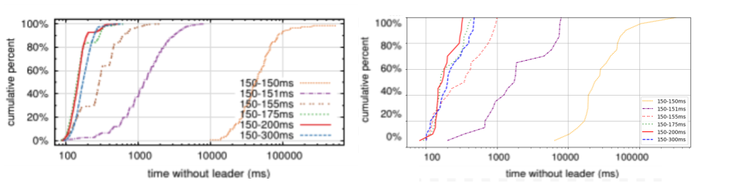
On Raft vs. Paxos
A main claim of the paper is that Raft was designed to be more understandable without sacrificing performance. Circumstantial industry trends and our own opinions formed through our replication efforts suggest that Raft is easier to understand for several reasons:
- Decomposition into Subtasks: Raft breaks down the consensus process into clear, manageable subtasks. This modularity makes it easier to grasp and implement.
- Strong Leadership Model: Raft’s strong leader model simplifies the process of achieving consensus, as there is a single point of authority for log replication and state changes.
We believe these features contribute to Raft’s increased understandability and effectiveness compared to Paxos, which handles nondeterminism through a sequence of proposals and acceptances, making it inherently more complex.
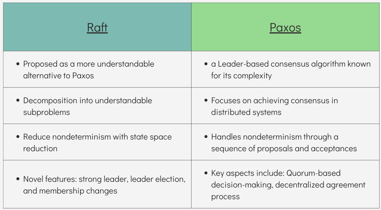
Discussion
The general trends of our results support the paper’s claim that randomized election timeouts are better for availability in comparison to a constant election timeout for every node. More anecdotally, we found that the use of random timeouts to determine which server would become the leader was easy to understand, especially compared to the other methods they discussed in the paper.
Similarly, based on our anecdotal experience, we believe the paper’s main claim that Raft is an easier to understand protocol than Paxos. However, the evidence presented in the paper is somewhat circumstantial, so we’d love to see a larger scale study proving this more concretely.
]]>Introduction
The paper “Formal Methods for Network Performance Analysis” by Mina Tahmasbi Arashloo, Ryan Beckett, and Rachit Agarwal, presented at the 20th USENIX Symposium on Networked Systems Design and Implementation (NSDI ’23), introduces a novel approach to analyzing network performance using formal methods. The authors demonstrate that it is possible to accurately model network components and their queues using first-order logic and leverage program synthesis techniques alongside SMT Solving to automatically generate concise, interpretable workloads for performance metric queries. This approach offers a significant advancement in network performance analysis tools, being more exhaustive than traditional simulation and emulation methods. It is also readily applicable to algorithms and protocols expressible in first-order logic. The effectiveness of this methodology is showcased through the analysis of packet scheduling algorithms and a small leaf-spine network, where it identifies potential issues with throughput, fairness, starvation, and latency.
The Claim Chosen for Replication
Among the results presented in the paper, we chose to replicate the plot (Figure 7c in the paper which is also shown below) illustrating the exponential growth of runtimes with increasing network size for a leaf-spine network. This particular figure was selected because evaluating exponential behavior through a graph provides clearer insights compared to interpreting numerical data from tables. Additionally, this was the only figure that included a table/graph for showing the results. The plot includes several curves corresponding to verification times, search time, base example generation time, etc. Our focus was on reconstructing the “query” using Z3’s C++ API, which plays a part in the “base example” generation time. Thus, we plot the “base example” curve and make a comparison with the original plot.

The x-axis of the figure above shows the size of the leaf-spine network under study. Si-Lj-Hk presents a leaf-spine network with i spines, j leaves, and k hosts. A sample leaf-spine network with 2 spines, 3 leaves, and 6 hosts is shown below:

Methodology Described in the Paper
The high-level approach outlined in the paper involves the following steps:
Defining a Mathematical Model of the Network: The authors introduce the concept of timed packet sequences to track how much time a packet spends inside a switch and the interactions of packets competing for resources:

To capture this concept, the authors introduce queuing modules as the basic building blocks of the network:

Each queueing module has some input queues, a processing block, and a number of output queues. These building blocks can be wired together in an arbitrary manner to model the desired network topology under study.
Specifying the Query: The query is a property that needs to be verified about the network under study. The property is typically on throughput, latency, and fairness. For example, a sample query on fairness can be:

where cenq (Q, t) and cdeq(Q, t) are the number of packets respectively enqueued into and dequeued from queue Q by the end of time t. The authors fully define the grammar supported by their framework in the paper.
Automatically Analyzing the Entire Input Space: This analysis occurs through an interactive process between the synthesis engine and the Z3 SMT Solver. The goal is to synthesize a workload representing a set of packet traces that satisfy the query. We do not mention the details of the synthesis algorithm here as they were not in the scope of our project.
Prove or Disprove the Property: If the formula “model AND base_wl AND wl AND (NOT query)” is SAT, it means an assignment to the formula is found, making it satisfiable. This indicates that the query was violated, meaning a set of packet traces violating the query has been found. If it is UNSAT, it means no such assignment is found, thus confirming that the query always holds.
Methodology Used
To remeasure the runtimes for creating the base examples, we wrote our own code to construct the expression corresponding to the leaf-spine network query using the C++ API of Z3. According to section 8 of the paper, the expression is a latency query:

The query asks whether the total number of packets received by host i at time 10 is less than half of what it should have received at the line rate. The base workload ensures that host 1 sends a steady stream of traffic to host 6 (at least 1 packet per time step), and no two hosts send traffic to the same destination so there is no traffic concentration at the hosts. The SMT-LIB representation of the query above is as follows:
(assert
  (=> (and
        (forall ((t Int))
          (and (>= t 1) (<= t 10) (= (dst 1 t) 6))
        )
        (forall ((i Int) (j Int))
          (=> (and (>= i 1) (<= i 6) (>= j 1) (<= j 6) (not (= i j)))
              (forall ((t Int))
                (and (>= t 1) (<= t 10) (not (= (dst i t) (dst j t))))
              )
          )
        )
      )
      (forall ((t Int))
        (and (>= t 1) (<= t 10) (< (cenq Out_6 t) 5))
      )
  )
)
We then integrated our code (which constructs the formula above using the C++ API of Z3) with the authors’ source code (fperf) written in C++, by making a call from their code to ours to obtain the corresponding Z3 expression. This expression was then used in their workflow. Once our code was integrated, we remeasured the runtime of the base example generation part and plotted it.
Results and Discussion
The result we obtained is shown in the following figure:

While we successfully illustrated the exponential behavior in the runtime, the runtimes still differed by approximately 15% for the same network sizes. We believe that this variance is natural in the realm of SMT solvers. Here is a more detailed discussion:
We did not have access to the exact hardware settings the authors used for their experiments. A better hardware setup is expected to lead to faster runtimes. Additionally, a recent paper, “Mariposa: Measuring SMT Instability in Automated Program Verification” (Technical Report) published in FMCAD 2023, introduces the performance instability problem in SMT Solvers (including Z3). This instability arises due to simple query mutations such as symbol renaming and randomness reseeding. Given that we do not know precisely how the authors constructed their query formula (e.g., the variable names they used) or what seed they employed, our formula could have differed from theirs, even though they are semantically equivalent, leading to different runtimes. To mitigate this possibility, we experimented with five different seeds and plotted the average runtime over all of them.
]]>