
Compared to the first edition from 2011 and the second edition from 2021, the book has been thoroughly revised. The code examples were updated to work with current LaTeX classes and packages as used in 2026, so everything compiles smoothly with modern distributions.
This edition also adds new material. There are chapters on creating presentation slides, a closer look at TeX engines and formats, and a section on using AI tools such as ChatGPT to speed up coding, reviewing, and even parts of the writing and publishing workflow.
The book now has about 400 pages and is printed in color, which helps especially with presentation examples and other colored output. As before, it focuses on hands-on examples that show how to structure documents, typeset mathematics, create tables and figures, manage citations and bibliographies, and produce professional PDFs for research papers, theses, or books.
There’s also a companion website at: https://latexguide.org
It hosts all code examples along with an integrated online LaTeX compiler, so you can run and edit the examples directly in your browser—even on a phone or tablet.
The book is available as a printed edition and as a Kindle ebook. If you buy either version, you can also download the DRM-free PDF for free from the publisher’s website: https://packt.link/free-ebook/9781805804574
About the author
Stefan Kottwitz has been active in the LaTeX community for many years, helping users online and building resources around the ecosystem. He has written more than 10,000 forum posts on LaTeX.org alone, providing support and advice to users worldwide.
He maintains several LaTeX community platforms, including the forums LaTeX.org and goLaTeX.de, and the Q&A sites TeXwelt.de and TeXnique.fr. He also runs the graphics gallery sites TeXample.net, TikZ.net, PGFplots.net, Asymp.net and FeynM.net. He runs CTAN LaTeX software mirrors in the EU, UK, US, and Japan, and the TeXdoc.org documentation service.
Stefan is a moderator on TeX Stack Exchange and matheplanet.com, and writes blog posts on LaTeX.net, TeX.co, and TeX-talk.net.
He distilled this experience into several books. In addition to the LaTeX Beginner’s Guide, he also wrote the LaTeX Cookbook and LaTeX Graphics with TikZ with Packt Publishing, both of which were also translated into Japanese by Asakura Publishing.
 Find the book here: packt.link/n96Mx For a short time, the third edition is 20% off for a limited number of copies.
Vortragsprogramm: https://www.dante.de/veranstaltungen/dante2026/
Für die Mitgliederversammlung am Samstag wird es einen anderen Videoraum geben. Zugangsdaten können vor Samstag, 08:30 Uhr, per Mail an [email protected] angefragt werden.
Vom 12.–14. März 2026 findet die DANTE-Frühjahrstagung 2026 in Lahnau statt. Alle, die sich für TeX, LaTeX, ConTeXt, Typografie und verwandte Themen interessieren und fachlichen wie persönlichen Austausch schätzen, sind herzlich willkommen!
Die Tagung läuft von Donnerstag bis Samstag, mit einem optionalen Einstieg schon am Mittwoch, 11. März, zu Einführungskursen und zum Vorabendtreff.
Der Veranstalter DANTE e.V. ist der deutschsprachige Verein für Anwender von TeX, LaTeX, ConTeXt und verwandten Themen, vom Einsteiger bis zum Profi.
Veranstaltungsort ist:
WIWA Wilhelm Wagner GmbH & Co. KG
Gewerbestraße 1–3
35633 Lahnau
Lahnau liegt zwischen Wetzlar und Gießen. Beide Städte sind gut per Bahn erreichbar. Von dort fahren die Buslinien 24 und 240 direkt in die Nähe des Tagungsortes.
Das Programm im Überblick
Mittwoch, 11. März 2026 (nachmittags)
- ConTeXt-Einführung (Hraban Ramm)
- LaTeX-Einführung (Philipp Kammerer)
(jeweils bis zu 3 Stunden, TeX Live sollte man bereits installiert haben) - Vorabendtreff zum lockeren Ankommen
Donnerstag, 12. März 2026
- 9:00–17:00 Uhr: Vortragsprogramm (im Aufbau, siehe unten)
- 19 Uhr Abendtreff
Freitag, 13. März 2026
- 9:30 Uhr: Werksführung bei Leica Camera
- 13:00–17:00 Uhr: Vortragsprogramm
- 19 Uhr Gemeinsames Tagungsessen
Samstag, 14. März 2026 (ab 9:00 Uhr)
- 68. Mitgliederversammlung von DANTE e.V.
(auch für interessierte Nicht-Mitglieder offen)
Hier ist schonmal eine Liste der bisher zugesagten Vorträge, noch ohne zeitliche Einordnung:
- samcarter — Zisterzienser Ziffern mit LaTeX (Lightning Talk)
Zisterzienser Ziffern sind ein Zahlensystem, das im Mittelalter von Mönchen
des Zisterzienserordens entwickelt wurde. Nach einer kurzen Einführung in
dieses heute fast vergessene Zahlensystem werden die LaTeX-Pakete
xistercian und cistercian vorgestellt, mit denen sich
Zisterzienser Ziffern in LaTeX darstellen lassen. - Marei Peischl & Patrick Gundlach — LaTeX und ZUGFeRD
Der Vortrag erklärt, was eine elektronische Rechnung nach EN 16931 ist,
welche Rolle ZUGFeRD dabei spielt und wie sich ZUGFeRD-Rechnungen mit LaTeX
erstellen und nutzen lassen. - Adelheid Bonnetsmüller — Having Fun With LaTeX XII
In der Vortragsreihe „Having Fun With LaTeX“ werden seit vielen Jahren kleinere
LaTeX-Pakete vorgestellt, die nützlich sind oder einfach Spaß machen – und in
jedem Fall zeigen, wie vielfältig das LaTeX-Universum ist. - Peter Turczak & Hraban Ramm — WIWAdoc – professioneller Textsatz im Unternehmen
Vorstellung der Firma WIWA sowie des LaTeX-basierten Dokumentationssystems
WIWAdoc für den professionellen Einsatz im Unternehmen. - Hraban Ramm — Datenzentrierte Dokumente mit ConTeXt
WIWA-Datenblätter werden aus verschiedenen Quellen wie CSV, JSON und Markdown
mithilfe von Lua in ConTeXt zusammengestellt. - Ulrike Fischer, LaTeX Team — (folgt)
- Frank Mittelbach, LaTeX Team — (folgt)
- Ulrik Vieth — OpenType Mathematikschriften: Was gibt es Neues?
Überblick über aktuell verfügbare OpenType-Mathematikschriften sowie über
neue Entwicklungen der letzten Zeit. - Marei Peischl — Engagement bei DANTE: wie und was?
- Stephan Lukasczyk & Adelheid Bonnetsmüller — Campai: Einblick in das neue Mitgliederverwaltungs- und Buchungsprogramm bei DANTE e.V.
Campai wird seit Ende 2023 für die Mitgliederverwaltung und seit 2025 für die
Buchhaltung bei DANTE e.V. eingesetzt. Der Vortrag stellt das System vor,
zeigt seine Funktionen und gibt Einblick in die praktische Arbeit damit.
Fragen und Diskussionen sind ausdrücklich willkommen.
Lust, selbst einen Vortrag zu halten? Es werden noch Beiträge gesucht, auch kurze Lightning Talks, sowohl zu TeX, LaTeX, ConTeXt, Schriftsatz, Schriftentwicklung, als auch zu angrenzenden Themen.
Alle Infos zu Anreise, Übernachtungsmöglichkeiten, genauen Zeiten, Kosten, und die Möglichkeit zur Einreichung von Vorträgen findest du hier: www.dante.de/veranstaltungen/dante2026/, und siehe auch die Einladung auf der tex-d-l Mailing-Liste.
Die Anmeldung ist bereits offen:
 www.dante.de/anmeldung-dante-2026
Neben all den Vorträgen und Workshops trifft man bekannte Gesichter wieder, lernt neue kennen und führt Gespräche, die man online so nicht hätte. Nach meiner Erfahrung ist alles sehr entspannt, offen und herzlich. Ich war schon öfter dabei, und habe früher auch manchmal Tagungsberichte hier und da notiert.
Bei Fragen kannst du dich auch direkt bei den Organisatoren melden: [email protected]
Bis dann!
]]>The Sri Yantra (also known as Sri Chakra or the Great Yantra) is one of the most mathematically complex geometric diagrams from ancient India, dating back to at least the 7th-8th century A.D. The earliest known specimens include a portrait in the Śrngari Matha (8th century A.D.) and mentions in Buddhist inscriptions from 7th century A.D. South Sumatra.

Here’s the code to look at and to test with the online compiler, and an explanation will follow:
\documentclass[tikz,border=2mm]{standalone}

\usetikzlibrary{backgrounds,math}

\begin{document}

\pgfdeclarelayer{minus1}
\pgfdeclarelayer{minus2}
\pgfdeclarelayer{minus3}
\pgfsetlayers{minus3,minus2,minus1,background,main}

\begin{tikzpicture}

% Base parameters
\def\cx{150}
\def\cy{150}
\def\scale{0.025}

\def\triangleData{%
  {53.65669559977147}{123.20508075688774}{250}{246.34330440022853}{0}% D1
  {52.984011026495736}{174.24660560764943}{50}{247.01598897350425}{1}% U1
  {98.71823312733801}{220.03828947357886}{123.20508075688774}{201.281766872662}{1}% U3
  {78.26467997914015}{197.92315674002487}{78.10499177949904}{221.73532002085986}{1}% U2
  {90.4856922951427}{78.10499177949904}{160.66014976539617}{209.51430770485734}{0}% D3
  {80.98384838952128}{103.12199145016105}{220.03828947357886}{219.0161516104787}{0}% D2
  {114.9488500600036}{160.66014976539617}{103.12199145016105}{185.0511499399964}{1}% U4
  {116.35142605010424}{134.30757626706648}{197.92315674002487}{183.64857394989576}{0}% D4
  {124.61190803072795}{144.79777263138968}{174.24660560764943}{175.38809196927207}{0}% D5
}

% Function to transform and draw triangle
% Usage: \drawtriangle{x1}{y1}{x2}{y2}{x3}{y3}
\newcommand{\drawtriangle}[6]{%
    \draw[thick] ({((#1-\cx)*\scale)},{(-(#2-\cy)*\scale)}) --
                 ({((#3-\cx)*\scale)},{(-(#4-\cy)*\scale)}) --
                 ({((#5-\cx)*\scale)},{(-(#6-\cy)*\scale)}) -- cycle;%
}

% Macro to draw a triangle from array data
% Arguments: left_x, top/base_y, center_y, right_x, type
\newcommand{\drawTriangleFromData}[5]{%
  \ifnum#5=0
    % Downward triangle: left_x, top_y, center_x, center_y, right_x, top_y
    \drawtriangle{#1}{#2}{\cx}{#3}{#4}{#2}%
  \else
    % Upward triangle: left_x, base_y, center_x, center_y, right_x, base_y
    \drawtriangle{#1}{#2}{\cx}{#3}{#4}{#2}%
  \fi
}

% Recursive macro to process triangle data
% Stops when it encounters \relax as the first argument
\def\processTriangleData#1#2#3#4#5{%
  \ifx\relax#1\relax
    % End of data reached
  \else
    \drawTriangleFromData{#1}{#2}{#3}{#4}{#5}%
    \expandafter\processTriangleData
  \fi
}

% Outer circle
\draw[thick, fill=white!30!white] (0,0) circle (2.5cm);

% Center bindu
\draw[fill=red] (0,0) circle (0.1cm);

% Draw all triangles from triangleData array
\expandafter\processTriangleData\triangleData\relax\relax\relax\relax\relax

%Step-11

\begin{scope}[on background layer]
\draw [fill=yellow] circle (3cm);

\foreach \i [evaluate=\i as \start using 22.5+45*\i] in {0,...,7}
	\draw[fill=green!30!black] (\start:2.5) .. controls ({\start-5}:2.85) and ({\start-17.5}:2.75) .. ({\start-22.5}:3) .. controls ({\start-27.5}:2.75) and ({\start-40}:2.85) .. ({\start-45}:2.5) arc [start angle={\start-45}, delta angle=45, radius=2.5cm]--cycle;
\end{scope}

%Step-12

\begin{pgfonlayer}{minus1}
\draw [fill=orange] circle (3.5cm);

\foreach \i [evaluate=\i as \start using 11.25+22.5*\i] in {0,...,15}
	\draw[fill=blue!30] (\start:3)  .. controls ({\start-2.5}:3.35) and ({\start-8.75}:3.25) .. ({\start-11.25}:3.5) .. controls ({\start-13.75}:3.25) and  ({\start-20}:3.35).. ({\start-22.5}:3) arc [start angle={\start-11.25}, delta angle=22.5, radius=3.5cm]--cycle;
\end{pgfonlayer}

%Step-13

\begin{pgfonlayer}{minus2}
\draw [fill=yellow!39] circle (4cm);
\draw [line width=2mm, blue!70!black] circle (3.75cm);
\end{pgfonlayer}

%Step-14

\begin{pgfonlayer}{minus3}
\node [fill=black, minimum size=8cm] (b) {};
\node [fill=black, minimum width=9.25cm, minimum height=3cm] (bh) {};
\node [fill=black, minimum height=9.25cm, minimum width=3cm] (bv) {};
\node [fill=black, minimum height=6mm, minimum width=6cm] at (bv.north) (bn) {};
\node [fill=black, minimum height=6mm, minimum width=6cm] at (bv.south) (bs) {};
\node [fill=black, minimum width=6mm, minimum height=6cm] at (bh.west) (bw) {};
\node [fill=black, minimum width=6mm, minimum height=6cm] at (bh.east) (be) {};
\draw [red!60!black,line width=1mm]%
(be.south west)-|(be.north east)-|(bh.north-|be.west)-|(b.north east)-|(bv.east|-bn.south)-|(bn.north east)-|(bn.south west)-|(b.north-|bv.west)-|(b.west|-bh.north)-|(bw.north east)-|(bw.south west)-|(bw.east|-bh.south)-|(b.south west)-|(bv.west|-bs.north)-|(bs.south west)-|(bs.north east)-|(bv.east|-b.south)-|(b.east|-bh.south)-|cycle;

\end{pgfonlayer}
\end{tikzpicture}
\end{document}
This work is derived partially from the above-mentioned research papers; however, the previous works contained several mathematical errors in coordinate calculations and failed to achieve precise superposition of intersection points, resulting in inaccurate triangle vertex positions. The previous interlockings resulted in holes within the intersections, where intersections formed polygons instead of precise points. This implementation corrects the above works and provides verified coordinates that ensure accurate interlocking of Sri Chakram with precise superposition of all nine triangles at all intersection points. While it is not possible to completely remove all errors in such a complex geometric construction, this work minimizes them to a negligible extent.
Mathematical Construction Complexity
The precise reproduction of the Sri Yantra central seal (14-angled polygon
composed by the intersection of nine triangles) is a highly difficult problem
that exceeds the capacity of hand-drawing. The structure consists of
- Nine interlocking triangles (4 upward, 5 downward) forming 43 smaller triangles through their intersections
- Most lines pass through 3-6 points of intersection, requiring precise superposition that is nearly impossible to achieve manually
The construction involves four structural components, each requiring iterative
procedures with three levels of enclosure. If we designate the number of
iterative steps for components 1-4 as a, b, c, d, respectively, the total
work required is: N = a*d + b*c*d + c*d + d.
This exponential growth in complexity makes accurate hand-drawing extremely
difficult, requiring computational assistance for precise construction.
Classification of Sri Yantra Types
Based on mathematical analysis of available specimens, three main types have
been identified:
Type I: Described by incomplete system of equations (2-3 equations from a
complete 4-equation system). Solutions are functions, allowing
continuous deformation. Most prevalent type (70% of specimens),
found in 17-19th century A.D., mostly on paper.
Type II: Also described by incomplete system (2-3 equations), allowing
continuous deformation. Some specimens are near the plane limits
of Type III. Found in 18-20th century A.D. (20% of specimens).
Type III: Described by complete system of 4 equations with 4 variables.
Solutions are discrete roots, making these portrayals rigid and
undeformable. Most mathematically precise type, found in specimens
from 17th century A.D. or earlier (10% of specimens), typically
on metal plates (cast) or stone. These may represent the original
prototype preserved through precise matrix-copying methods.
Type III₁: A special linear case of Type III, where points C and D are
strictly fixed at the outer circumference.
Spherical vs. Plane Construction Theory
Some rare specimens (Type III variants) use arcs of ovals or ellipses instead
% of straight lines, suggesting they may be plane projections of a spherical
image. The spherical construction theory proposes:
- The outer circumference is formed by a side cross-section of a sphere
- Triangle sides are geodesic lines on the sphere (formed by central
cross-sections) - The position is determined by an angle α relative to the sphere’s axis
- As α → 0, the spherical image transforms to its linear limit (Type III₁)
Mathematical Analysis
The general analytical aspect of the polygon requires solving systems of
linear and circular equations with coordinate superposition. Type III and
Type III₁ portrayals are described by complete systems of equations, making
them mathematically rigid. Type I and II portrayals, being described by
incomplete systems, allow continuous deformation and may represent
simplifications that arose from centuries-old accumulation of copying errors.
The investigation of Type III₁ seals has not revealed correlations expressed
in whole numbers, vulgar fractions, or well-known transcendental constants,
indicating the mathematical relationships are more complex than simple
geometric ratios.
Historical Development
The mathematical sequence Type III → Type III₁ → Type II → Type I represents
a progression from general to special cases. This suggests Type III may be
the hypothetical original, with others being successive simplifications
resulting from copying errors over centuries. The prevalence of simpler,
more contemporary types (I and II) supports this theory, as they were
produced using less precise drawing instruments compared to the casting
methods used for Type III specimens.
References:
- Kulaichev, A.P. (1984). “Sriyantra and its Mathematical Properties.”
Journal of Indian Philosophy, 12(2), 161-184.
Available at: http://protein.bio.msu.ru/~akula/Kulaichev%20math.pdf - Huet, G. “Sri Yantra: Construction and Mathematical Properties.”
ResearchGate publication.
Available at: https://www.researchgate.net/profile/Gerard-Huet/publication/277295011_Sri_Yantra/links/55af62d008aed9b7dcddbc42/Sri-Yantra.pdf
Methodology
- Define Base Parameters:
– Establish center coordinates (cx, cy) and scale factor for coordinate
transformation from original SVG coordinates to the TikZ coordinate system
– Original coordinate system: center at (150, 150), radius 100
– TikZ coordinate system: center at (0, 0), radius 2.5cm
– Scale factor: 2.5/100 = 0.025
– Y-axis transformation: y_tikz = -(y_original – 150) * 0.025 - Calculate Triangle Coordinates:
– Define coordinates for all nine triangles using precise geometric
calculations derived from line-line intersection formulas
– Each triangle is defined by three vertices:
* Downward triangles (D1-D5): left_x, top_y, center_y, right_x, top_y
* Upward triangles (U1-U4): left_x, base_y, center_y, right_x, base_y
– Store coordinates as variables using \pgfmathsetmacro for proper
expansion in mathematical expressions - Implement Drawing Function:
– Create \drawtriangle macro that takes 6 parameters (x1, y1, x2, y2,
x3, y3) representing three vertices
– Apply coordinate transformation to convert from the original coordinate
system to TikZ coordinate system
– Draw a closed triangle path using \draw command - Draw All Components:
– Draw outer circle (boundary of the yantra)
– Draw center bindu (red dot at origin)
– Draw all nine triangles using the \drawtriangle function with
calculated coordinates
– Draw decorative elements (lotus petals, bhupura) on background layers
Mathematical Formulation for Coordinate Derivation:
1. Triangle Edge Line Equations:
For a triangle with vertices P₁(x₁, y₁), P₂(x₂, y₂), P₃(x₃, y₃):
Edge P₁P₂:
If x₁ ≠ x₂: y = m₁₂(x – x₁) + y₁, where m₁₂ = (y₂ – y₁)/(x₂ – x₁)
If x₁ = x₂: x = x₁ (vertical line)
Edge P₂P₃:
If x₂ ≠ x₃: y = m₂₃(x – x₂) + y₂, where m₂₃ = (y₃ – y₂)/(x₃ – x₂)
If x₂ = x₃: x = x₂ (vertical line)
Edge P₃P₁:
If x₃ ≠ x₁: y = m₃₁(x – x₃) + y₃, where m₃₁ = (y₁ – y₃)/(x₁ – x₃)
If x₃ = x₁: x = x₃ (vertical line)
2. Line-Line Intersection Formula:
Given two lines:
L₁: y = m₁x + c₁ (or x = k₁ for vertical)
L₂: y = m₂x + c₂ (or x = k₂ for vertical)
Intersection point I(xᵢ, yᵢ):
Case 1: Both lines non-vertical (m₁ ≠ ∞, m₂ ≠ ∞):
xᵢ = (c₂ – c₁)/(m₁ – m₂), provided m₁ ≠ m₂
yᵢ = m₁xᵢ + c₁ = m₂xᵢ + c₂
Case 2: L₁ vertical (x = k₁), L₂ non-vertical:
xᵢ = k₁
yᵢ = m₂k₁ + c₂
Case 3: L₂ vertical (x = k₂), L₁ non-vertical:
xᵢ = k₂
yᵢ = m₁k₂ + c₁
Case 4: Both vertical (x = k₁, x = k₂):
If k₁ = k₂: Lines coincide (infinite intersections)
If k₁ ≠ k₂: Lines parallel, no intersection
3. System of Equations for Sri Yantra:
For 9 triangles with 27 edges total, we have:
Let Tᵢ (i = 1 to 9) represent the i-th triangle with vertices:
Tᵢ = {Vᵢ₁(xᵢ₁, yᵢ₁), Vᵢ₂(xᵢ₂, yᵢ₂), Vᵢ₃(xᵢ₃, yᵢ₃)}
Each triangle has 3 edges Eᵢⱼ (j = 1, 2, 3):
Eᵢ₁: edge from Vᵢ₁ to Vᵢ₂
Eᵢ₂: edge from Vᵢ₂ to Vᵢ₃
Eᵢ₃: edge from Vᵢ₃ to Vᵢ₁
For each intersection point Iₖ where edges Eᵢⱼ and Eₚᵩ intersect:
Iₖ = Intersection(Eᵢⱼ, Eₚᵩ)
The system requires that all intersection points are precisely
superposed, meaning:
For any two edges Eᵢⱼ and Eₚᵩ that should intersect at point P:
Distance(Intersection(Eᵢⱼ, Eₚᵩ), P) < ε (where ε is negligible)
4. Geometric Constraints:
a) Symmetry constraint (vertical axis at x = 150):
For triangle Tᵢ with left vertex (xₗ, y) and right vertex (xᵣ, y):
xₗ + xᵣ = 2 × 150 = 300
xᵣ = 300 – xₗ
b) Triangle vertex constraints:
Each triangle vertex must lie on the triangle’s edges:
For triangle Tᵢ with vertices Vᵢ₁, Vᵢ₂, Vᵢ₃:
Vᵢ₁ ∈ Eᵢ₃ (lies on edge from Vᵢ₃ to Vᵢ₁)
Vᵢ₂ ∈ Eᵢ₁ (lies on edge from Vᵢ₁ to Vᵢ₂)
Vᵢ₃ ∈ Eᵢ₂ (lies on edge from Vᵢ₂ to Vᵢ₃)
c) Intersection point constraints:
When multiple edges intersect at the same point P(xₚ, yₚ):
For all edges Eᵢⱼ passing through P:
P ∈ Eᵢⱼ (point P satisfies the line equation of Eᵢⱼ)
5. Optimization Objective:
Minimize the total error function:
E = Σᵢⱼₚᵩ |Distance(Intersection(Eᵢⱼ, Eₚᵩ), Expected_Point)|
Subject to constraints:
- All triangle vertices satisfy triangle edge equations
- Symmetry is maintained (xₗ + xᵣ = 300)
- All intersection points are precisely superposed
- No gaps or polygons at intersection points
6. Iterative Solution Method:
Using Newton-Raphson or similar iterative method:
Step 1: Initialize triangle parameters (centers, scales, orientations)
Step 2: Calculate all edge equations
Step 3: Compute all intersection points
Step 4: Calculate error E
Step 5: If E > ε:
- Compute gradient ∂E/∂parameters
- Update parameters: params_new = params_old – α·∇E
- Return to Step 2
- Else:
– Solution converged
Where α is the learning rate and ε is the convergence threshold.
7. Final Coordinate Values:
The coordinates listed below are the solutions to this system,
obtained through the iterative refinement process, ensuring:
- Precise superposition at all intersection points
- No holes or polygon formations
- Symmetry around x = 150
- Errors minimized to a negligible extent
Triangle coordinates (solutions to the mathematical system above)
Store coordinates in a structured way
Triangle data: {left_x, top/base_y, center_y, right_x, type}
type: 0 = downward (uses top_y), 1 = upward (uses base_y)
Bhaskar Tripathi, PhD (Financial Mathematics), https://www.bhaskartripathi.com
]]>
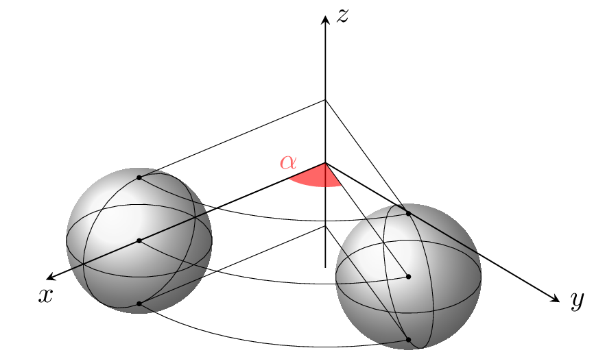
You can specify any angle. Invisible line segments are drawn as dashed lines.
Edit and compile if you like:
\documentclass{beamer}
\usepackage{tikz}
\usepackage{tikz-3dplot}
\usepackage{ifthen}

% beamer settings
\definecolor{blackboard}{HTML}{00552E}
\setbeamercolor{background canvas}{bg=blackboard}

\begin{document}

\newcommand{\hexprism}[2]{
\tdplotsetmaincoords{#1}{#2}
\colorlet{maincolor}{white}
\begin{tikzpicture}[
tdplot_main_coords,
axis/.style={-stealth},
mainline/.style={maincolor,very thick,line join=bevel},
invisibleline/.style={maincolor,densely dashed},
]

\pgfmathsetmacro{\r}{1} % Length of a side of the bottom
\pgfmathsetmacro{\h}{4} % height

\foreach \P/\ang in{A/0,B/60,C/120,D/180,E/240,F/300}
\coordinate (\P b) at (\ang:\r);

\foreach \P/\ang in{A/0,B/60,C/120,D/180,E/240,F/300}
\coordinate (\P t) at ({\r*cos(\ang)},{\r*sin(\ang)},\h);

\foreach \P in{A,B,C,D,E,F}
{\node[maincolor!50!gray] at(\P t){\scriptsize \P t};
\node[maincolor!50!gray] at(\P b){\scriptsize \P b};
}

\tikzset{
  ABrec/.style={insert path={(Ab)--(Bb)--(Bt)--(At)--cycle}},
  BCrec/.style={insert path={(Bb)--(Cb)--(Ct)--(Bt)--cycle}},
  CDrec/.style={insert path={(Cb)--(Db)--(Dt)--(Ct)--cycle}},
  DErec/.style={insert path={(Db)--(Eb)--(Et)--(Dt)--cycle}},
  EFrec/.style={insert path={(Eb)--(Fb)--(Ft)--(Et)--cycle}},
  FArec/.style={insert path={(Fb)--(Ab)--(At)--(Ft)--cycle}},
}

% camera vector: ({sin(\tdplotmaintheta)*sin(\tdplotmainphi)},{-sin(\tdplotmaintheta)*cos(\tdplotmainphi)},{cos(\tdplotmaintheta)})
% inner product
% side inner product
\pgfmathparse{cos(30)*sin(\tdplotmaintheta)*sin(\tdplotmainphi)-sin(30)*sin(\tdplotmaintheta)*cos(\tdplotmainphi) >= 0}
\pgfmathsetmacro{\ABprod}{\pgfmathresult}
\pgfmathparse{cos(90)*sin(\tdplotmaintheta)*sin(\tdplotmainphi)-sin(90)*sin(\tdplotmaintheta)*cos(\tdplotmainphi) >= 0}
\pgfmathsetmacro{\BCprod}{\pgfmathresult}
\pgfmathparse{cos(150)*sin(\tdplotmaintheta)*sin(\tdplotmainphi)-sin(150)*sin(\tdplotmaintheta)*cos(\tdplotmainphi) >= 0}
\pgfmathsetmacro{\CDprod}{\pgfmathresult}
\pgfmathparse{cos(210)*sin(\tdplotmaintheta)*sin(\tdplotmainphi)-sin(210)*sin(\tdplotmaintheta)*cos(\tdplotmainphi) >= 0}
\pgfmathsetmacro{\DEprod}{\pgfmathresult}
\pgfmathparse{cos(270)*sin(\tdplotmaintheta)*sin(\tdplotmainphi)-sin(270)*sin(\tdplotmaintheta)*cos(\tdplotmainphi) >= 0}
\pgfmathsetmacro{\EFprod}{\pgfmathresult}
\pgfmathparse{cos(330)*sin(\tdplotmaintheta)*sin(\tdplotmainphi)-sin(330)*sin(\tdplotmaintheta)*cos(\tdplotmainphi) >= 0}
\pgfmathsetmacro{\FAprod}{\pgfmathresult}

% bottom inner product
\pgfmathparse{cos(\tdplotmaintheta) >= 0}
\pgfmathsetmacro{\topprod}{\pgfmathresult}

\ifthenelse{
    \topprod=1
}{\draw[mainline](At)--(Bt)--(Ct)--(Dt)--(Et)--(Ft)--cycle;
    \ifthenelse{\ABprod=1 \and \BCprod=1 \and \CDprod=1}{
        \draw[invisibleline](Db)--(Eb)--(Fb)--(Ab); \draw[invisibleline](Eb)--(Et) (Fb)--(Ft);
        \draw[mainline,ABrec];\draw[mainline,BCrec];\draw[mainline,CDrec];
    }{ \ifthenelse{\BCprod=1 \and \CDprod=1 \and \DEprod=1}{
        \draw[invisibleline](Eb)--(Fb)--(Ab)--(Bb); \draw[invisibleline](Fb)--(Ft) (Ab)--(At);
        \draw[mainline,BCrec];\draw[mainline,CDrec];\draw[mainline,DErec];
    }{\ifthenelse{\CDprod=1 \and \DEprod=1 \and \EFprod=1}{
        \draw[invisibleline](Fb)--(Ab)--(Bb)--(Cb); \draw[invisibleline](Ab)--(At) (Bb)--(Bt);
        \draw[mainline,CDrec];\draw[mainline,DErec];\draw[mainline,EFrec];
    }{\ifthenelse{\DEprod=1 \and \EFprod=1 \and \FAprod=1}{
        \draw[invisibleline](Ab)--(Bb)--(Cb)--(Db); \draw[invisibleline](Bb)--(Bt) (Cb)--(Ct);
        \draw[mainline,DErec];\draw[mainline,EFrec];\draw[mainline,FArec];
    }{\ifthenelse{\EFprod=1 \and \FAprod=1 \and \ABprod=1}{
        \draw[invisibleline](Bb)--(Cb)--(Db)--(Eb); \draw[invisibleline](Cb)--(Ct) (Db)--(Dt);
        \draw[mainline,EFrec];\draw[mainline,FArec];\draw[mainline,ABrec];
    }{\ifthenelse{\FAprod=1 \and \ABprod=1 \and \BCprod=1}{
        \draw[invisibleline](Cb)--(Db)--(Eb)--(Fb); \draw[invisibleline](Db)--(Dt) (Eb)--(Et);
        \draw[mainline,FArec];\draw[mainline,ABrec];\draw[mainline,BCrec];
    }{}}}}}}
}{\draw[mainline](Ab)--(Bb)--(Cb)--(Db)--(Eb)--(Fb)--cycle;
    \ifthenelse{\ABprod=1 \and \BCprod=1 \and \CDprod=1}{
        \draw[invisibleline](Dt)--(Et)--(Ft)--(At); \draw[invisibleline](Eb)--(Et) (Fb)--(Ft);
        \draw[mainline,ABrec];\draw[mainline,BCrec];\draw[mainline,CDrec];
    }{ \ifthenelse{\BCprod=1 \and \CDprod=1 \and \DEprod=1}{
        \draw[invisibleline](Et)--(Ft)--(At)--(Bt); \draw[invisibleline](Fb)--(Ft) (Ab)--(At);
        \draw[mainline,BCrec];\draw[mainline,CDrec];\draw[mainline,DErec];
    }{\ifthenelse{\CDprod=1 \and \DEprod=1 \and \EFprod=1}{
        \draw[invisibleline](Ft)--(At)--(Bt)--(Ct); \draw[invisibleline](Ab)--(At) (Bb)--(Bt);
        \draw[mainline,CDrec];\draw[mainline,DErec];\draw[mainline,EFrec];
    }{\ifthenelse{\DEprod=1 \and \EFprod=1 \and \FAprod=1}{
        \draw[invisibleline](At)--(Bt)--(Ct)--(Dt); \draw[invisibleline](Bb)--(Bt) (Cb)--(Ct);
        \draw[mainline,DErec];\draw[mainline,EFrec];\draw[mainline,FArec];
    }{\ifthenelse{\EFprod=1 \and \FAprod=1 \and \ABprod=1}{
        \draw[invisibleline](Bt)--(Ct)--(Dt)--(Et); \draw[invisibleline](Cb)--(Ct) (Db)--(Dt);
        \draw[mainline,EFrec];\draw[mainline,FArec];\draw[mainline,ABrec];
    }{\ifthenelse{\FAprod=1 \and \ABprod=1 \and \BCprod=1}{
        \draw[invisibleline](Ct)--(Dt)--(Et)--(Ft); \draw[invisibleline](Db)--(Dt) (Eb)--(Et);
        \draw[mainline,FArec];\draw[mainline,ABrec];\draw[mainline,BCrec];
    }{}}}}}}
}
\end{tikzpicture}
}

\foreach \a in{0,5,...,360}{
\begingroup
\begin{frame}
\centering
  \hexprism{70}{\a}
\end{frame}
\endgroup
}

\foreach \a in{70,75,...,430}{
\begingroup
\begin{frame}
\centering
  \hexprism{\a}{5}
\end{frame}
\endgroup
}

\end{document}
]]>
Edit and compile if you like:
\documentclass{article}
\usepackage{tikz}
\usepackage{tikz-3dplot}
\usepackage{ifthen}
\begin{document}
\newcommand{\tetrahedron}[3][(0,0,0)]{
\tdplotsetmaincoords{#2}{#3}
\begin{tikzpicture}[
maincolor/.style=cyan,
scale=1.5,
tdplot_main_coords,
axis/.style={-stealth},
mainline/.style={maincolor,thick},
invisibleline/.style={cyan,densely dashed},
]
% axis
\draw[axis](-1.5,0,0)--(1.5,0,0)node[pos=1.1]{$x$};
\draw[axis](0,-1.5,0)--(0,1.5,0)node[pos=1.1]{$y$};
\draw[axis](0,0,-1)--(0,0,2)node[pos=1.1]{$z$};

% vertices
\coordinate[shift={#1}] (A) at (60:1);
\coordinate[shift={#1}] (B) at (180:1);
\coordinate[shift={#1}] (C) at (300:1);
\coordinate[shift={#1}] (O) at (0,0,{sqrt(2)});

% fill faces
\fill[maincolor,opacity=0.1](A)--(B)--(C)--cycle;
\fill[maincolor,opacity=0.1](O)--(B)--(C)--cycle;
\fill[maincolor,opacity=0.1](A)--(O)--(C)--cycle;
\fill[maincolor,opacity=0.1](A)--(B)--(O)--cycle;

% inner product
\pgfmathparse{-sin(\tdplotmaintheta)*sin(\tdplotmainphi)+(1+cos(60))*sin(\tdplotmaintheta)*cos(\tdplotmainphi)/sin(60)+cos(\tdplotmaintheta)/sqrt(2)>0}
\pgfmathsetmacro{\OBCprod}{\pgfmathresult}
\pgfmathparse{-sin(\tdplotmaintheta)*sin(\tdplotmainphi)-(1+cos(60))*sin(\tdplotmaintheta)*cos(\tdplotmainphi)/sin(60)+cos(\tdplotmaintheta)/sqrt(2)>0}
\pgfmathsetmacro{\OABprod}{\pgfmathresult}
\pgfmathparse{sin(\tdplotmaintheta)*sin(\tdplotmainphi)/cos(60)+cos(\tdplotmaintheta)/sqrt(2)>0}
\pgfmathsetmacro{\OCAprod}{\pgfmathresult}
\pgfmathparse{-cos(\tdplotmaintheta)>0}
\pgfmathsetmacro{\ABCprod}{\pgfmathresult}

\ifthenelse{\ABCprod=0 \and \OABprod=0 \and \OBCprod=0 \and \OCAprod=1}{
\draw[invisibleline](O)--(B) (A)--(B) (C)--(B); \draw[mainline](A)--(O)--(C)--cycle; % 0001
}{
\ifthenelse{\ABCprod=0 \and \OABprod=0 \and \OBCprod=1 \and \OCAprod=0}{
\draw[invisibleline](O)--(A) (B)--(A) (C)--(A); \draw[mainline](O)--(B)--(C)--cycle; % 0010
}{
\ifthenelse{\ABCprod=0 \and \OABprod=0 \and \OBCprod=1 \and \OCAprod=1}{
\draw[mainline](O)--(C) (O)--(A)--(C) (O)--(B)--(C);\draw[invisibleline](A)--(B); % 0011
}{
\ifthenelse{\ABCprod=0 \and \OABprod=1 \and \OBCprod=0 \and \OCAprod=0}{
\draw[invisibleline](O)--(C) (A)--(C) (C)--(B); \draw[mainline](A)--(B)--(O)--cycle; % 0100
}{
\ifthenelse{\ABCprod=0 \and \OABprod=1 \and \OBCprod=0 \and \OCAprod=1}{
\draw[mainline](O)--(A) (O)--(B)--(A) (O)--(C)--(A);\draw[invisibleline](B)--(C); % 0101
}{
\ifthenelse{\ABCprod=0 \and \OABprod=1 \and \OBCprod=1 \and \OCAprod=0}{
\draw[mainline](O)--(B) (O)--(A)--(B) (O)--(C)--(B);\draw[invisibleline](A)--(C); % 0110
}{
\ifthenelse{\ABCprod=0 \and \OABprod=1 \and \OBCprod=1 \and \OCAprod=1}{
\draw[mainline](O)--(A) (O)--(B) (O)--(C) (A)--(B)--(C)--cycle; % 0111
}{
\ifthenelse{\ABCprod=1 \and \OABprod=0 \and \OBCprod=0 \and \OCAprod=0}{
\draw[invisibleline](O)--(A) (O)--(B) (O)--(C); \draw[mainline](A)--(B)--(C)--cycle; % 1000
}{
\ifthenelse{\ABCprod=1 \and \OABprod=0 \and \OBCprod=0 \and \OCAprod=1}{
\draw[mainline](A)--(C) (A)--(O)--(C) (A)--(B)--(C);\draw[invisibleline](O)--(B); % 1001
}{
\ifthenelse{\ABCprod=1 \and \OABprod=0 \and \OBCprod=1 \and \OCAprod=0}{
\draw[mainline](B)--(C) (B)--(A)--(C) (B)--(O)--(C);\draw[invisibleline](A)--(O); % 1010
}{
\ifthenelse{\ABCprod=1 \and \OABprod=0 \and \OBCprod=1 \and \OCAprod=1}{
\draw[mainline](O)--(A) (O)--(B) (O)--(C) (A)--(B)--(C)--cycle; % 1011
}{
\ifthenelse{\ABCprod=1 \and \OABprod=1 \and \OBCprod=0 \and \OCAprod=0}{
\draw[mainline](A)--(B) (A)--(C)--(B) (A)--(O)--(B);\draw[invisibleline](C)--(O); % 1100
}{
\ifthenelse{\ABCprod=1 \and \OABprod=1 \and \OBCprod=0 \and \OCAprod=1}{
\draw[mainline](O)--(A) (O)--(B) (O)--(C) (A)--(B)--(C)--cycle; % 1101
}{
\ifthenelse{\ABCprod=1 \and \OABprod=1 \and \OBCprod=1 \and \OCAprod=0}{
\draw[mainline](O)--(A) (O)--(B) (O)--(C) (A)--(B)--(C)--cycle; % 1110
}{%
}}}}}}}}}}}}}}

% draw points
\foreach \P in{A,B,C,O}
\path(0,0,{sqrt(2)/3})--(\P)node[pos=1.2]{\P};
\end{tikzpicture}
}

\tetrahedron{60}{35}

\end{document}

Edit and compile if you like:
\documentclass{article}
\usepackage{tikz}
\usepackage{tikz-3dplot}
\usepackage{ifthen}
\usepackage{tcolorbox}
\tcbuselibrary{most}
\usepackage[top=30truemm,bottom=30truemm,left=17truemm,right=17truemm]{geometry}

\begin{document}
\newcommand{\tetrahedron}[3][(0,0,0)]{
\tdplotsetmaincoords{#2}{#3}
\begin{tikzpicture}[
maincolor/.style=cyan,
scale=1.5,
tdplot_main_coords,
axis/.style={-stealth},
mainline/.style={maincolor,thick},
invisibleline/.style={cyan,densely dashed},
]
% axis
\draw[axis](-1.5,0,0)--(1.5,0,0)node[pos=1.1]{$x$};
\draw[axis](0,-1.5,0)--(0,1.5,0)node[pos=1.1]{$y$};
\draw[axis](0,0,-1)--(0,0,2)node[pos=1.1]{$z$};

% vertices
\coordinate[shift={#1}] (A) at (60:1);
\coordinate[shift={#1}] (B) at (180:1);
\coordinate[shift={#1}] (C) at (300:1);
\coordinate[shift={#1}] (O) at (0,0,{sqrt(2)});

% fill faces
\fill[maincolor,opacity=0.1](A)--(B)--(C)--cycle;
\fill[maincolor,opacity=0.1](O)--(B)--(C)--cycle;
\fill[maincolor,opacity=0.1](A)--(O)--(C)--cycle;
\fill[maincolor,opacity=0.1](A)--(B)--(O)--cycle;

% inner product
\pgfmathparse{-sin(\tdplotmaintheta)*sin(\tdplotmainphi)+(1+cos(60))*sin(\tdplotmaintheta)*cos(\tdplotmainphi)/sin(60)+cos(\tdplotmaintheta)/sqrt(2)>0}
\pgfmathsetmacro{\OBCprod}{\pgfmathresult}
\pgfmathparse{-sin(\tdplotmaintheta)*sin(\tdplotmainphi)-(1+cos(60))*sin(\tdplotmaintheta)*cos(\tdplotmainphi)/sin(60)+cos(\tdplotmaintheta)/sqrt(2)>0}
\pgfmathsetmacro{\OABprod}{\pgfmathresult}
\pgfmathparse{sin(\tdplotmaintheta)*sin(\tdplotmainphi)/cos(60)+cos(\tdplotmaintheta)/sqrt(2)>0}
\pgfmathsetmacro{\OCAprod}{\pgfmathresult}
\pgfmathparse{-cos(\tdplotmaintheta)>0}
\pgfmathsetmacro{\ABCprod}{\pgfmathresult}

\ifthenelse{\ABCprod=0 \and \OABprod=0 \and \OBCprod=0 \and \OCAprod=1}{
\draw[invisibleline](O)--(B) (A)--(B) (C)--(B); \draw[mainline](A)--(O)--(C)--cycle; % 0001
}{
\ifthenelse{\ABCprod=0 \and \OABprod=0 \and \OBCprod=1 \and \OCAprod=0}{
\draw[invisibleline](O)--(A) (B)--(A) (C)--(A); \draw[mainline](O)--(B)--(C)--cycle; % 0010
}{
\ifthenelse{\ABCprod=0 \and \OABprod=0 \and \OBCprod=1 \and \OCAprod=1}{
\draw[mainline](O)--(C) (O)--(A)--(C) (O)--(B)--(C);\draw[invisibleline](A)--(B); % 0011
}{
\ifthenelse{\ABCprod=0 \and \OABprod=1 \and \OBCprod=0 \and \OCAprod=0}{
\draw[invisibleline](O)--(C) (A)--(C) (C)--(B); \draw[mainline](A)--(B)--(O)--cycle; % 0100
}{
\ifthenelse{\ABCprod=0 \and \OABprod=1 \and \OBCprod=0 \and \OCAprod=1}{
\draw[mainline](O)--(A) (O)--(B)--(A) (O)--(C)--(A);\draw[invisibleline](B)--(C); % 0101
}{
\ifthenelse{\ABCprod=0 \and \OABprod=1 \and \OBCprod=1 \and \OCAprod=0}{
\draw[mainline](O)--(B) (O)--(A)--(B) (O)--(C)--(B);\draw[invisibleline](A)--(C); % 0110
}{
\ifthenelse{\ABCprod=0 \and \OABprod=1 \and \OBCprod=1 \and \OCAprod=1}{
\draw[mainline](O)--(A) (O)--(B) (O)--(C) (A)--(B)--(C)--cycle; % 0111
}{
\ifthenelse{\ABCprod=1 \and \OABprod=0 \and \OBCprod=0 \and \OCAprod=0}{
\draw[invisibleline](O)--(A) (O)--(B) (O)--(C); \draw[mainline](A)--(B)--(C)--cycle; % 1000
}{
\ifthenelse{\ABCprod=1 \and \OABprod=0 \and \OBCprod=0 \and \OCAprod=1}{
\draw[mainline](A)--(C) (A)--(O)--(C) (A)--(B)--(C);\draw[invisibleline](O)--(B); % 1001
}{
\ifthenelse{\ABCprod=1 \and \OABprod=0 \and \OBCprod=1 \and \OCAprod=0}{
\draw[mainline](B)--(C) (B)--(A)--(C) (B)--(O)--(C);\draw[invisibleline](A)--(O); % 1010
}{
\ifthenelse{\ABCprod=1 \and \OABprod=0 \and \OBCprod=1 \and \OCAprod=1}{
\draw[mainline](O)--(A) (O)--(B) (O)--(C) (A)--(B)--(C)--cycle; % 1011
}{
\ifthenelse{\ABCprod=1 \and \OABprod=1 \and \OBCprod=0 \and \OCAprod=0}{
\draw[mainline](A)--(B) (A)--(C)--(B) (A)--(O)--(B);\draw[invisibleline](C)--(O); % 1100
}{
\ifthenelse{\ABCprod=1 \and \OABprod=1 \and \OBCprod=0 \and \OCAprod=1}{
\draw[mainline](O)--(A) (O)--(B) (O)--(C) (A)--(B)--(C)--cycle; % 1101
}{
\ifthenelse{\ABCprod=1 \and \OABprod=1 \and \OBCprod=1 \and \OCAprod=0}{
\draw[mainline](O)--(A) (O)--(B) (O)--(C) (A)--(B)--(C)--cycle; % 1110
}{%
}}}}}}}}}}}}}}

% draw points
\foreach \P in{A,B,C,O}
\path(0,0,{sqrt(2)/3})--(\P)node[pos=1.2]{\P};
\end{tikzpicture}
}

\begin{tcbitemize}[
    raster equal height=rows,
    raster columns=3,
    colframe=black!70!blue,
    colback=white,
    sharp corners,
    ]
\tcbitem[title={\centering$\theta=60,\phi=35$}]\centering
\tetrahedron{60}{35}

\tcbitem[title={\centering$\theta=60,\phi=80$}]\centering
\tetrahedron{60}{80}

\tcbitem[title={\centering$\theta=60,\phi=120$}]\centering
\tetrahedron{60}{120}

\tcbitem[title={\centering$\theta=60,\phi=35$}]\centering
\tetrahedron{30}{35}

\tcbitem[title={\centering$\theta=60,\phi=80$}]\centering
\tetrahedron{20}{80}

\tcbitem[title={\centering$\theta=60,\phi=120$}]\centering
\tetrahedron{30}{120}
\end{tcbitemize}

\end{document}
]]>
Edit and compile if you like:
\documentclass{standalone}
\usepackage{tikz}
\usetikzlibrary{calc}

\begin{document}

\def\angle{70} % launch angle
\def\v{6}   % initial velocity
\def\g{9.8} % gravitational acceleration
\def\r{0.1} % ball radius

\begin{tikzpicture}[
    scale=4,
    axis/.style={-stealth},
]

    \pgfmathsetmacro{\tGround}{{2*\v*sin(\angle)/\g}}
    \newcommand{\Ballx}[1]{{\v*#1*\tGround*cos(\angle)}}
    \newcommand{\Bally}[1]{{-0.5*\g*#1*#1*\tGround*\tGround+\v*#1*\tGround*sin(\angle)}}

    % Axis
    \draw[axis] (-0.3,0) -- ($1.2*(\Ballx{1},0)$) node[right] {$x$};
    \draw[axis] (0,-0.3) -- ($1.2*(0,\Bally{0.5})$) node[above] {$y$};

    % Angle
    \filldraw[opacity=0.5] (\r*1.6,0) arc(0:\angle:\r*1.6)node[opacity=1,midway,above right]{$\theta$} -- (0,0) -- cycle;

    % Ball
    \newcommand{\DrawBall}[2][black]{
        \filldraw[ball color=#1!50!] (\Ballx{#2},\Bally{#2}) circle(\r);
        \draw[-stealth,#1] (\Ballx{#2},\Bally{#2})
            --++({0.1*\v*cos(\angle)}, {-0.1*\g*#2*\tGround + 0.1*\v*sin(\angle)}); % velocity
    }

    \foreach \t in {0,0.2,0.8,1} {
        \DrawBall[black]{\t}
    }

    \draw[densely dotted] (\Ballx{0.2},0) node[below] {$x=v_0t\cos\theta$}
        -- (\Ballx{0.2},\Bally{0.2})
        -- (0,\Bally{0.2}) node[left] {$\displaystyle y=-\frac{1}{2}gt^2+v_0t\sin\theta$};

    \DrawBall[red]{0.5}

    % Trajectory
    \draw[samples=256,densely dotted,domain=0:1,variable=\t] plot(\Ballx{\t},\Bally{\t});

\end{tikzpicture}
\end{document}
]]>
Edit and compile if you like:
\documentclass{standalone}
\usepackage{tikz}
\usepackage{tikz-3dplot}
\usetikzlibrary{calc,backgrounds}

\begin{document}
\tdplotsetmaincoords{60}{140}
\begin{tikzpicture}[
    tdplot_main_coords,
    scale=3,
    axis/.style={-stealth},
    addline/.style={very thin}
]

    \begin{scope}[axis]
        \draw (0,0,0) -- (1.5,0,0) node[below]{$x$};
        \draw (0,0,0) -- (0,1.5,0) node[right]{$y$};
        \draw (0,0,-0.5) -- (0,0,0.7) node[right]{$z$};
    \end{scope}

    \def\r{0.3} % radius of sphere
    \def\a{70} % rotation angle

    \coordinate (A) at (1,0,0);
    \coordinate (B) at ({cos(\a)},{sin(\a)},0);
    \foreach \P/\Ptop/\Pbottom in {A/Atop/Abottom, B/Btop/Bbottom} {
        \coordinate (\Ptop) at ($(\P)+(0,0,\r)$);
        \coordinate (\Pbottom) at ($(\P)+(0,0,-\r)$);
    }

    % rotation angle
    \fill[red, opacity=0.6] (0.2,0) node[above]{$\alpha$}
        arc [radius=0.2, start angle=0, end angle=\a] -- (0,0,0) -- cycle;

    % draw additional line
    \begin{scope}[addline]
        \draw (A) circle (\r);
        \draw (B) circle (\r);
        \foreach \h in {-\r,0,\r}
            \draw (1,0,\h) arc [radius=1, start angle=0, end angle=\a] -- (0,0,\h) -- cycle;

        \tdplotsetrotatedcoords{\a-90}{90}{0}
        \tdplotdrawarc[tdplot_rotated_coords]{(B)}{\r}{0}{360}{}{}

        \tdplotsetrotatedcoords{90}{90}{0}
        \tdplotdrawarc[tdplot_rotated_coords]{(A)}{\r}{0}{360}{}{}
    \end{scope}

    %point and sphere
    \begin{scope}[tdplot_screen_coords, on background layer]
        \fill[ball color=lightgray!20!] (A) circle (\r);
        \fill[ball color=lightgray!20!] (B) circle (\r);
        \foreach \P in {A,B,Atop,Btop,Abottom,Bbottom}
            \fill (\P) circle (0.01);
    \end{scope}
\end{tikzpicture}
\end{document}
]]>2024年11月に、Stefan Kottwitz著のTikZに関する書籍の翻訳版が朝倉書店から発売されました。LaTeXで画像を作るための実用的な入門書。TikZにより数学、科学、技術論文に図や画像を簡単に入れられる。アイデアやデータを可視化してプロフェッショナルな図表やプロットを2次元でも3次元でも表示できるようになるために。

本書の内容
第1章「TikZで始める」はTikZ入門だ。他のグラフィックスパッケージと比較してTikZの利点を論じる。TikZとは何かという全体像と独特の哲学を理解する。TikZをインストールする方法を学び、簡単な図を作成していく。さらに、TikZや他のパッケージのマニュアルなどを参照するための役立つヒントが得られる。
第2章「TikZで最初の画像を作る」では、LaTeX文書を一から作る。TikZの構文を理解して、2 次元および3 次元のデカルト座標と極座標を学ぶ。さらに、基本的な多角形の作り方、画像での色の使い方を学ぶ。
第3章「ノードの位置決めと描画」ではノードという基本的概念を与える。様々な形態のノードを位置決めして並べ、テキスト、画像、ラベルを追加する方法を学ぶ。
第4章「辺と矢印を描く」では、ノードの間を辺、直線、曲線、矢印でつなぐ方法を示す。辺にテキストラベルをつける方法や並べ方、位置、方向を調整する方法を学ぶ。線のスタイルや矢頭の形状をカスタマイズしたり両方向にする方法も学ぶ。
第5章「スタイルと画像の読み込み」では、TikZ要素をグローバルまたはローカルなstyleで定義して使う方法を学ぶ。ノードと辺でスタイルを使う方法とスコープを使って画像全体や画像の一部に対してスタイルを適用する方法を学ぶ。さらに、ミニTikZ画像を他の画像の構成要素として使う方法も学ぶ。
第6章「木とグラフの描画」では、親子の階層関係を表す木構造を作る方法を示す。アイデアを可視化するマインドマップの描き方やグラフを生成する簡潔な構文を与える。さらに、LaTeXのtabular環境と同様な行列形式にオブジェクトを配置する方法も示す。/p>
第7章「塗りつぶし、クリッピング、シェーディング」では、より高度な技法から始める。複雑なパスで塗りつぶす方法、特定の領域の画像をクリップしたり、ある色から別の色になめらかに色を変える方法を学ぶ。
第8章「パスの豊かな表現」では、線を曲げたりジグザグにしたり波打たせるようなクリエイティブな効果を加える技法を学ぶ。テキストを曲線に沿わせたり、1 つのパスに複数の作用を適用する方法も学ぶ。
第9章「レイヤー、オーバーレイ、透明性を使う」では、様々なレイヤーに描画して、オブジェクトをテキストや画像の背後に置く方法を学ぶ。透明性を使ってこの効果を上げる方法も学ぶ。さらに、TikZのビジュアルな注釈を通常のLaTeX文書にスーパーインポーズしたり、透かしのような背景画像を追加したりする方法を学ぶ。
第10章「座標とパスで計算する」では、TikZで座標値を計算する効率的な方法を示す。この章は座標計算、距離や射影を使った座標の計算、パスの交点の計算を扱う。また、repeatコマンドでループしてコードを簡単にする方法を学ぶ。
第11章「座標とキャンバスを変換する」では、変換による移動、回転、拡大縮小に焦点を絞る。図に対してちょっとした手直しや複雑な変更を加える必要がある場合に、適切な調整や位置変更ができるスキルを学ぶ。
第12章「なめらかな曲線を描く」では簡単な曲線の曲がりを変えたり、なめらかにして角の尖りをなくし、手書きのように簡単に曲線を描く様々な方法を学ぶ。
第13章「2Dおよび3Dでのプロット」では、座標系でデータをプロットする方法を扱う。2Dおよび3Dでデカルト座標と極座標の座標軸のカスタマイズ、凡例の追加、パラメトリック曲線のプロット、プロットの交点の計算、プロットの間の色塗りを扱う。
第14章「各種チャートを描く」では、フローチャート、関係図、説明図、数量を表す図の作り方を学ぶ。図全体を自動的に作れるようにパッケージの活用法を学ぶ。
第15章「TikZで楽しもう」では、スキルの高いTikZユーザが追加パッケージのプログラミングを楽しみTikZコミュニティでシェアする方法などを列挙する。かわいい動物、人物、国旗、パズルやゲームを描画する方法も学ぶ。
]]>
The revised chapters have been rearranged, and a new chapter about using ChatGPT as a coding assistant and editing tool has been added. The new contents are as follows:
Chapter 1, Exploring Various Document Classes, gives insight into diverse document types, and you’ll discover how LaTeX is versatile for creating theses, books, CVs, presentations, flyers, and large posters with tailored examples.
Chapter 2, Tuning the Text, focuses on customizing text details within documents. Beginning with essential fundamentals, we’ll cover practical tips and conclude the chapter with demonstrations of LaTeX’s capabilities beyond standard paragraph formatting.
Chapter 3, Adjusting Fonts, shows how to make global font choices and explore techniques for adjusting fonts within your document.
Chapter 4, Creating Tables, explains how to craft visually appealing tables. This includes guidance on creating legible tables, aligning numeric data, and incorporating colors. It introduces the concept of floating tables and figures, enabling automated positioning. Additionally, the chapter discusses advanced topics such as merging and splitting cells and importing table data from external files.
Chapter 5, Working with Images, begins by exploring considerations related to image quality. You’ll find practical instructions on incorporating, positioning, shaping, and aligning images in LaTeX.
Chapter 6, Creating Graphics, provides step-by-step instructions for crafting compelling graphics. The chapter leverages modern graphics packages, enabling the creation of comprehensive graphics, including various types of diagrams and charts.
Chapter 7, Creating Beautiful Designs, guides you on incorporating background images, crafting attractive ornaments, integrating appealing headings, generating calendars and word clouds, incorporating symbols for computer keys and menu items, and simulating terminal output.
Chapter 8, Producing Contents, Indexes, and Bibliographies, provides practical solutions for quickly customizing the table of contents, lists of figures and tables, bibliographies, glossaries, and indexes.
Chapter 9, Optimizing PDF Files, explores the functionalities of PDFs, including metadata, PDF comments, and fillable forms. You’ll learn techniques for merging PDF files, adjusting margins, optimizing output for e-books, and creating animations in a PDF.
Chapter 10, Writing Advanced Mathematics, works with LaTeX’s enduring strengths—its exceptional typesetting capabilities for mathematical formulas. After a quick tutorial, you’ll learn advanced techniques for refining formulas and creating theorems, diagrams, geometric figures, and plots in 2D and 3D.
Chapter 11, Using LaTeX in Science and Technology, deals with additional scientific fields, including chemistry, physics, computer science, and various technologies such as electronics. This chapter provides a comprehensive overview, showcasing how LaTeX can be effectively applied across diverse fields through specific examples.
Chapter 12, Getting Support on the Internet, starts with a guide to the most valuable Internet resources for LaTeX. Then, it demonstrates how to seek support from the TeX online communities efficiently.
Chapter 13, Using Artificial Intelligence with LaTeX, provides guidance and examples on harnessing the capabilities of ChatGPT to streamline code work and enhance your content efficiently.
The book grew to 424 pages and is now printed in color for the best experience with the many drawings. It is also available as a Kindle book, and if you buy the printed book or the Kindle, you can get the PDF ebook for free at the publisher’s website.
]]>
This is a drawing of Totoro, the star of the Japanese animated fantasy film "My Neighbor Totoro".
The Koch snowflake fractal has been used to draw snow, repetitive tasks are done in "foreach" loops.

Edit and compile if you like:
% Totoro sitting in the snow
% By Noa Hoffmann and Pascal Günthner, 21.12.2020
\documentclass[tikz,11pt]{{standalone}}
\usepackage{calligra}
\usepackage[T1]{fontenc}
\usetikzlibrary{%
  shapes, shadows, patterns, calc,
  decorations.shapes,
  decorations.fractals,
  decorations.markings,
  decorations.pathmorphing
}

\colorlet{bodycolor}{black!35!gray!60!brown!98!green}
\colorlet{bellycolor}{yellow!70!white!92!green}

\tikzset{
   furspot/.pic = {
    \path [draw = black, thick, fill] (0,0)
    .. controls +(0.3,0)        and  +(0.25,-0.05)   ..  ++(0.35,-.45)
    .. controls +(-0.45,0.25)   and  +(0.1,0)        ..  ++(-0.85,-0.05)
    .. controls +(-0.3,0.1)     and  +(-0.4, 0)      ..  cycle;
   },
   claw/.pic = {
    \path [fill = bodycolor!70, draw] (0,0) arc (0:45:0.2 and 0.8)
                                           arc (135:180:0.2 and 0.8)
    arc (180:360:0.059) -- cycle;
   },
   whiskers/.pic = {
    \path [fill = bodycolor!70,draw] (0,0) arc (0:45:0.05 and 2.3)
                                        arc (135:180:0.3 and 2.3)
    to[out=-90,in=-90] cycle;
   },
   snowflake/.pic = {
   \fill [decoration = Koch snowflake, white] decorate{ decorate{
          decorate{ (-0.5,-0.3) -- ++(60:1) -- ++(-60:1) -- cycle }}};
   \foreach \i in {30, 90, 150, 210, 270, 330} {
        \draw[blue!50!white,very thin] (0,0) -- +(\i:0.3);
        }
    \draw[decoration = Koch snowflake, blue!50!white, very thin]
          decorate{($(0,0)+(60:0.2)$) -- ($(0,0)+(300:0.2)$) --
                   ($(0,0)+(180:0.2)$) -- cycle};
   }
}
\tikzset{
  snow/.style   = {decoration = {random steps, segment length = 2mm,
                   amplitude = 0.4mm}, decorate},
  plush/.style  = {decoration = {random steps, segment length = 1mm,
                   amplitude = 0.5mm},decorate}
}

\begin{document}
\begin{tikzpicture}[color = bodycolor, draw = black, thick]

%---------------------background and tail----------------------
% blue sky
\fill[blue!30!white] (-8cm,-11cm) rectangle (8cm,10cm);
% random snowflakes
\foreach \i in {0.1,0.11,...,1}{
  \pic [scale = \i, opacity = 0.9] at (rand*7.5, rnd*18-10.5) {snowflake};}
% more tiny snowflakes
\foreach \i in {0.1,0.11,...,0.5}{
  \pic [scale = \i, opacity = 0.9] at (rand*7.5, rnd*18-10.5) {snowflake};}
% cloud with merry christmas
\node [cloud,aspect = 6.5, cloud puff arc = 120, cloud puffs = 12.9, fill = white,
       color = white] at (0,7) {\Huge M \hspace{9.8cm}.};
\node [color = red] at (0,7) {\fontsize{50}{80}
                              \textbf{Merry Christmas \quad }};
% tail
\path [draw, fill, rotate = 50] (-4,-7.5) circle (1.5 and 2.2);
% snowhill
\fill [draw, gray!6, snow] (-8,-11) to[in=200, out=0] (-3,-7.5) to (3,-7.5)
      to[out=-20, in=180] (8,-11);

%--------------------body-----------------------------------------
% right ear
\path [fill, draw] (0.6,2.3)+(-45:1) arc (-60:35:1 and 1.5)
                   arc (115:210:1 and 1.5);
% left ear
\path [fill, draw] (-0.6,2.3)+(-135:1) arc (-120:-215:1 and 1.5)
                   arc (65:-30:1 and 1.5);
% head
\path [draw, fill] ($(0,0)+(170:2.5 and 2)$) arc (170:10:2.5 and 2)
                   arc(35:-20: 3 and 2)
        -- ($(0,-0.8)+(200:3 and 2)$) arc (200:145:3 and 2) -- cycle;
% body
\path[fill] ($(0,-4)+(200:4 and 4.5)$) arc (200:-20:4 and 4.5);

%----------------------face----------------------------------------
% left eye
\path [draw, fill = white] (-1.4,0.7) circle (0.45 and 0.4);
\fill [black] (-1.2,0.7) circle (0.16);
\fill [white] (-1.24,0.74) circle (0.03);
% right eye
\path [draw, fill = white, thick] (1.4,0.7) circle (0.4);
\fill [black] (1.25,0.7) circle (0.16);
\fill [white] (1.20,0.74) circle (0.03);
% nose
\path [draw] (0.35, 0.7) .. controls (0.2,0.8) and (-0.2, 0.8)
                         .. (-0.35, 0.7);
\path [fill = black] (0, 0.53) -- (0.25, 0.6)
      .. controls (0.3,0.75) and (-0.3, 0.75)
      .. (-0.25, 0.6) -- cycle;
\pic [scale = 0.3] at (0,0.8) {snowflake};
% mouth
\draw (-0.05,-0.5) arc (140:85:0.2 and 0.1);
% whiskers
\foreach \i/\j/\k/\l/\m in
    {80/1/1.5/-2/0,
    -90/-1/1.5/-2.2/-0.2,
    -80/-0.8/1.5/-2.5/-0.5,
    -80/1/1.3/2.2/0,
    90/-1/1.3/2.4/-0.2,
    80/-1/1.3/2.6/-0.4}
  \pic [rotate = \i, scale = \j, yscale = \k] at (\l,\m) {whiskers};

%-----------------------------arms----------------------------------
% handclaws
\foreach \i in {-4,-3.8,-3.6,3.9,3.7,3.5} { \pic [rotate = 180]
  at (\i,-6.5) {claw};}
% left arm
\path [draw, fill] (-3, -1) .. controls (-5.5,-3.5) and (-4.5,-7.5)
                            .. (-3.35,-6.45);
% right arm
\path [draw, fill] (3, -1)  .. controls (5.5,-3.5) and (4.5,-7.5)
                            .. (3.35,-6.45);

%------------------------belly----------------------------------
\draw[fill = bellycolor] ($(0,-4.7)+(230:3.8 and 4)$)
             to [out = -10,in = 190] ($(0,-4.7)+(-50:3.8 and 4)$)
             to ($(0,-4)+(-50:4.5)$)
             to [out = 60, in = -70] ($(0,-4.7)+(50:3.8 and 4)$)
             arc (50:130:3.8 and 4)
             to [out = -110, in = 120] ($(0,-4)+(-130:4.5)$)
             to cycle;
% fur spots
\foreach \i/\j/\k in {0/0/-1.3, -15/1.6/-1.5, 15/-1.6/-1.5,
    -8/0.7/-2.2, 8/-0.7/-2.2, -22/2.2/-2.5, 22/-2.2/-2.5} {
  \pic [rotate = \i] at (\j, \k) {furspot};}

%------------------------legs and feet--------------------------
%legs
\path [draw, rotate =  32, fill] (-5.8,-5.2) circle (0.9 and 1.4);
\path [draw, rotate = -32, fill] (5.8,-5.2) circle (0.9 and 1.4);
% left feet
\path [draw, fill, rotate =  30] (-5.6,-6.1) circle (0.65 and 0.6);
\path [draw, fill, rotate = -30] (5.6,-6.1) circle (0.65 and 0.6);
% toe beans
\path [draw, fill = bodycolor!50!white, rotate =  45] (-7,-4.7)
  circle (0.3 and 0.17);
\path [draw ,fill = bodycolor!50!white, rotate = -45] (7,-4.7)
  circle (0.3 and 0.17);
% footclaws
\foreach \i/\j/\k in {50/-2.2/-7.9,40/-2/-7.7,30/-1.75/-7.55,
    -50/2.3/-8,-40/2.1/-7.8,-30/1.85/-7.65} {
  \pic [rotate = \i] at (\j,\k) {claw};}

% hat
\path [draw, fill = red] (43:2.5) to [in = -170, out = 130] ($(0.7,3)+(195:0.4)$)
  to [in = 180, out = 90] (0.7,3.1) to [out = 150, in = 0] (0,3.3)
  to [in = 50, out = 180] (137:2.5);
\fill [draw, plush, fill = white, thin] (145:2.5 and 2) to [in = 160, out = 20]
  (35:2.5 and 2)
  to [out = 80, in = -80] ++(0,0.5) to [out = 160, in = 20] ($(145:2.5 and 2) +(0,0.5)$)
  to [in = 100, out = -100] cycle;
\fill [draw, plush, fill = white, thin] (0.7,3.1) circle (0.5);
\end{tikzpicture}
\end{document}
Click to download: totoro.tex • totoro.pdf
Open in Overleaf: totoro.tex ]]>
An animation to the area of calculation using the upper Riemann sum.
That's an approximation of an integral by a finite sum, named after the German mathematician Riemann. It is calculated by partitioning the region below the the curve into rectangles and summarizing their areas. To get a better approximation, the region is devided more finely. As the rectangles get smaller, the Rieman sum approaches the Riemann integral. This animation shows it.

Edit and compile if you like:
% Animation for Upper Riemann Sum
% Author: Edson José Teixeira
\documentclass[10pt]{beamer}
\usepackage[controls]{animate}
\usepackage{tikz}
\usetikzlibrary{arrows}
% Beamer Settings
\usetheme{Warsaw}
% Counters
\newcounter{higher}
\setcounter{higher}{1}
\begin{document}
\begin{frame}[fragile]{Upper Riemann Sum}
  \begin{figure}
    \begin{animateinline}[poster = first, controls]{5}
      \whiledo{\thehigher<30}{
        \begin{tikzpicture}[line cap=round, line join=round, >=triangle 45,
                            x=4.0cm, y=1.0cm, scale=1]
          \draw [->,color=black] (-0.1,0) -- (2.5,0);
          \foreach \x in {1,2}
            \draw [shift={(\x,0)}, color=black] (0pt,2pt)
                  -- (0pt,-2pt) node [below] {\footnotesize $\x$};
          \draw [color=black] (2.5,0) node [below] {$x$};
          \draw [->,color=black] (0,-0.1) -- (0,4.5);
          \foreach \y in {1,2,3,4}
            \draw [shift={(0,\y)}, color=black] (2pt,0pt)
                  -- (-2pt,0pt) node[left] {\footnotesize $\y$};
          \draw [color=black] (0,4.5) node [right] {$y$};
          \draw [color=black] (0pt,-10pt) node [left] {\footnotesize $0$};
          \draw [domain=0:2.2, line width=1.0pt] plot (\x,{(\x)^2});
          \clip(0,-0.5) rectangle (3,5);
          \draw (2,0) -- (2,4);
          \foreach \i in {1,...,\thehigher}
            \draw [fill=black,fill opacity=0.3, smooth,samples=50] ({1+(\i-1)/\thehigher},{(1+(\i)/\thehigher)^2})
                  --({1+(\i)/\thehigher},{(1+(\i)/\thehigher)^2})
                  --  ({1+(\i)/\thehigher},0)
                  -- ({1+(\i-1)/\thehigher},0)
                  -- cycle;
        \end{tikzpicture}
        %
        \stepcounter{higher}
        \ifthenelse{\thehigher<30}{ \newframe }{\end{animateinline} }
      }
      \caption{Upper Riemann Sum}
  \end{figure}
\end{frame}
\end{document}
Click to download: upper-riemann-sum.tex • upper-riemann-sum.pdf
Open in Overleaf: upper-riemann-sum.tex ]]>
An animation to the area of calculation using the lower Riemann sum.
That's an approximation of an integral by a finite sum, named after the German mathematician Riemann. It is calculated by partitioning the region below the the curve into rectangles and summarizing their areas. To get a better approximation, the region is devided more finely. As the rectangles get smaller, the Rieman sum approaches the Riemann integral.

Edit and compile if you like:
% Animation for Lower Riemann Sum
% Author: Edson José Teixeira
\documentclass[10pt]{beamer}
\usepackage[controls]{animate}
\usepackage{tikz}
\usetikzlibrary{arrows}
% Beamer Settings
\usetheme{Warsaw}
% Counters
\newcounter{lower}
\setcounter{lower}{1}
\begin{document}
\begin{frame}[fragile]{Lower Sum of Riemann}
  \begin{figure}
    \begin{animateinline}[poster = first, controls]{5}
    \whiledo{\thelower<30}{
      \begin{tikzpicture}[line cap=round, line join=round, >=triangle 45,
                          x=4.0cm, y=1.0cm, scale=1]
        \draw[->, color=black] (-0.1,0) -- (2.5,0);
        \foreach \x in {1,2}
          \draw [shift={(\x,0)}, color=black] (0pt,2pt)
                -- (0pt,-2pt) node [below] {\footnotesize $\x$};
        \draw [color=black] (2.5,0) node [below] {$x$};
        \draw [->, color=black] (0,-0.1) -- (0,4.5);
        \foreach \y in {1,2,3,4}
          \draw [shift={(0,\y)}, color=black] (2pt,0pt)
                -- (-2pt,0pt) node[left] {\footnotesize $\y$};
        \draw [color=black] (0,4.5) node [right] {$y$};
        \draw [color=black] (0pt,-10pt) node [left] {\footnotesize $0$};
        \draw [domain=0:2.2, line width=1.0pt] plot (\x,{(\x)^2});
        \clip (0,-0.5) rectangle (3,5);
        \draw (2,0)--(2,4);
        \foreach \i in {1,...,\thelower}
        \draw [fill=black, fill opacity=0.3, smooth,samples=50]
                 ({1+(\i-1)/\thelower}, {(1+(\i-1)/\thelower)^2})
              -- ({1+(\i)/\thelower},   {(1+(\i-1)/\thelower)^2})
              -- ({1+(\i)/\thelower},0)
              -- ({1+(\i-1)/\thelower},0)
              -- cycle;
      \end{tikzpicture}
      \stepcounter{lower}
      \ifthenelse{\thelower<30}{ \newframe }{\end{animateinline} }
    }
    \caption{Lower Riemann Sum}
  \end{figure}
\end{frame}
\end{document}
Click to download: lower-riemann-sum.tex • lower-riemann-sum.pdf
Open in Overleaf: lower-riemann-sum.tex ]]>
An isometric view of a random city.

Edit and compile if you like:
% Random city
% Author: Pascal Seppecher
\documentclass[tikz,border=10pt]{standalone}
\usetikzlibrary{backgrounds}
\usepackage{ifthen}
% The blue print color
\definecolor{blueprintcolor}{RGB}{20,20,100}

% The shadow color
\colorlet{shadow}{blueprintcolor!50!white}

% The light color
\colorlet{light}{white!90!blueprintcolor}

% The background color
\colorlet{background}{blueprintcolor}

% The basic size of a block
\newcommand\defaultside{0.6}

% The height of a storey
\newcommand\floorheight{0.08}

% The minimum number of stories
\newcommand\storeymin{20}

% The maximum number of stories
\newcommand\storeymax{40}

% The width of a window
\newcommand\window{0.05}

% The angles of x,y-axes
\newcommand\xaxis{210}
\newcommand\yaxis{-30}

% Facade style random list
\pgfmathdeclarerandomlist{facade}{{\hlines}{\vlines}{\grid}{\grid}{\grid}}

% Vertical thickness
\newcommand\vthickness{thin}

% Horizontal thickness
\newcommand\hthickness{thin}

% Selects at random the thickness of the horizontal lines
\newcommand\setvthickness{
  \pgfmathrandominteger{\alea}{0}{3}
  \ifthenelse{\alea=0}{\renewcommand\vthickness{thick}}{}
  \ifthenelse{\alea=1}{\renewcommand\vthickness{thin}}{}
  \ifthenelse{\alea=2}{\renewcommand\vthickness{very thin}}{}
  \ifthenelse{\alea=3}{\renewcommand\vthickness{ultra thin}}{}
}

% Selects at random the thickness of the vertical lines
\newcommand\seththickness{
  \pgfmathrandominteger{\alea}{0}{3}
  \ifthenelse{\alea=0}{\renewcommand\hthickness{thick}}{}
  \ifthenelse{\alea=1}{\renewcommand\hthickness{thin}}{}
  \ifthenelse{\alea=2}{\renewcommand\hthickness{very thin}}{}
  \ifthenelse{\alea=3}{\renewcommand\hthickness{ultra thin}}{}
}

% Draws vertical lines on each side of the block
\newcommand\vlines[2]{
  \pgfmathsetmacro\size{#1 * \floorheight}
  \pgfmathsetmacro\max{#2/\window}
  \foreach \col in {1,...,\max}
  {
    \pgfmathsetmacro\xx{-\col * \window}
    \draw[\vthickness,draw=shadow, shift={(\yaxis:\xx)}] (0,0)--(0,\size);
    \draw[\vthickness,draw=light, shift={(\xaxis:\xx)}] (0,0)--(0,\size);
  }
}

% Draws horizontal lines on each side of the block
\newcommand\hlines[2]{
  \foreach \floor in {0,...,#1}
  {
    \pgfmathsetmacro\z{\floor * \floorheight}
    \draw[\hthickness,draw=shadow, shift={(90:\z)}] (150:#2)--(0,0);
    \draw[\hthickness,draw=light, shift={(90:\z)}] (0,0) -- (30:#2);
  }
}

% Draws horizontal and vertical lines on each side of the block
\newcommand\grid[2]{
  \vlines{#1}{#2}
  \hlines{#1}  {#2}
}

% Draws a block at the specified position
\newcommand\block[2]{
  % Computes the height of the block
  \pgfmathsetmacro\height{#2 * \floorheight}

  % Erases the background
  \fill[fill=background]
    (0,0) -- (150:#1) -- ++(0,\height) -- (0,\height) -- (0,0);
  \fill[fill=background]
    (0,0) -- (30:#1) -- ++(0,\height) -- (0,\height) -- (0,0);

  % Draws the facades
  \facade{\stories}{#1}

  % Frames the facades
  \draw[draw=shadow] (0,0) -- (150:#1) -- ++(0,\height) -- (0,\height) -- (0,0);
  \draw[draw=light] (0,0) -- (30:#1) -- ++(0,\height) -- (0,\height) -- (0,0);

  % Draws the terrace
  \fill[fill=background, draw=light,shift={(90:\height)}]
    (0,0) -- (30:#1) -- (0,#1) --(150:#1)--(0,0);

  %
  \pgfmathrandominteger{\alea}{0}{3}
  \ifthenelse{\alea=0}{
  % Sometimes, adds more stores (= skyscraper)
    \begin{scope}[shift={(0,\height)},shift={(0,0.05)}]
      \pgfmathsetmacro\pside{#1-0.1}
      \pgfmathrandominteger{\stories}{2}{\storeymax}
      \block{\pside}{\stories}
    \end{scope}
  }{}

  \ifthenelse{\alea=1}{
  % Sometimes, draws a pyramid roof
  \pyramid{\height}{#1}
  }{}
}

% Draws a basic block
\newcommand\basicblock[3]{
  % Selects a random facade style
  \pgfmathrandomitem{\facade}{facade}
  \setvthickness{}
  \seththickness{}

  % Selects a random number of stores
  \pgfmathrandominteger{\stories}{\storeymin}{\storeymax}

  \begin{scope}[shift={(\xaxis:#1)},shift={(\yaxis:#2)}]
  \block{#3}{\stories}
  \end{scope}
}

% Draws a pyramid roof
\newcommand\pyramid[2]{
  % Computes the side of the pyramid
  \pgfmathsetmacro\pside{#2-0.1}

  % Selects the height of the pyramid at random
  \pgfmathparse{random()}
  \pgfmathsetmacro\top{0.5+\pgfmathresult/3}

  % Draws the pyramid
  \begin{scope}[fill=background, draw=light,shift={(90:#1)},shift={(90:0.05)}]
    \fill[draw=light] (0,0) -- (30:\pside) -- (0,\top) -- (150:\pside)--(0,0);
    \draw (0,0) -- (0,\top);
  \end{scope}
}

% Draws a random city of the specified dimensions
\newcommand\city[2]{
  \foreach \x in {1,...,#1}
    \foreach \y in {1,...,#2}
      {\basicblock{\x}{\y}{\defaultside}}
}

\begin{document}
% Draws a hundred blocks random city
\begin{tikzpicture}[show background rectangle,
  background rectangle/.style={fill=background}]
    \city{10}{10}
\end{tikzpicture}
\end{document}
Click to download: city.tex • city.pdf
Open in Overleaf: city.tex ]]>
This diagram is for the Bernoulli Principle in physics.
See:
- https://en.wikipedia.org/wiki/File:BernoullisLawDerivationDiagram.svg
- https://en.wikipedia.org/wiki/Bernoulli%27s_principle (Derivations of the Bernoulli equation)

Edit and compile if you like:
% Diagram for the Bernoulli Principle
% Author: Roland Puntaier
\documentclass[tikz,border=10pt]{standalone}
\usetikzlibrary{calc}
\begin{document}
\begin{tikzpicture}
  \def\XSTART{0}
  \def\YSTART{3}
  \def\YDIAONE{2.5}
  \def\YDIATWO{2}
  \def\YCURVE{2}
  \def\XCURVE{2}
  \def\XEND{15}
  \def\XONESTART{2}
  \def\XONEDELTA{2}
  \def\DD{0.5}

  \def\YEND{\YSTART+\YCURVE+\YDIATWO}
  \def\XCURVESTART{\XEND/2-\XSTART/2-\XCURVE/2}
  \def\XCURVESTARTUP{\XEND/2-\XSTART/2-\XCURVE}
  \def\XCURVEEND{\XEND/2-\XSTART/2 + \XCURVE/2}
  \def\XONEEND{\XONESTART+\XONEDELTA}
  \def\XTWOSTART{\XCURVEEND+\XONESTART}
  \def\XTWODELTA{\XONEDELTA*\YDIAONE*\YDIAONE/\YDIATWO/\YDIATWO}
  \def\XTWOEND{\XTWOSTART+\XTWODELTA}
  \def\YTWOMIDDLE{\YSTART+\YCURVE+\YDIATWO/2}
  \def\YONEMIDDLE{\YSTART+\YDIAONE/2}
  \def\GROUND{\YSTART/4}

  \tikzset{
      partial ellipse/.style args={#1:#2:#3}{
          insert path={+ (#1:#3) arc (#1:#2:#3)}
      },
      dimen/.style={<->,>=latex,thin,
        every rectangle node/.style={fill=white,midway,font=\sffamily}},
  }

  \draw (\XSTART,\YSTART) -- (\XCURVESTART,\YSTART)
    to[out=0, in=180, looseness=0.75]
      (\XCURVEEND,{\YSTART+\YCURVE}) -- (\XEND,{\YSTART+\YCURVE});
  \draw (\XSTART,{\YSTART+\YDIAONE}) -- (\XCURVESTARTUP,{\YSTART+\YDIAONE})
    to[out=0, in=180, looseness=0.75] (\XCURVEEND,\YEND) -- (\XEND,\YEND);

  \draw [fill=gray] (\XONESTART,\YSTART) coordinate (BA)
    rectangle (\XONEEND,{\YSTART+\YDIAONE}) coordinate (BB);
  \draw [fill=lightgray](\XONESTART,\YONEMIDDLE) node [below] {$A_1$}
    ellipse ({\YDIAONE/6} and {\YDIAONE/2});
  \draw [fill=gray,dashed](\XONEEND,\YONEMIDDLE)
    ellipse ({\YDIAONE/6} and {\YDIAONE/2});
  \draw (\XONEEND,\YONEMIDDLE)
    [partial ellipse=-90:90:{\YDIAONE/6} and {\YDIAONE/2}];

  \draw [fill=gray] (\XTWOSTART,{\YSTART+\YCURVE}) coordinate (CA)
    rectangle (\XTWOEND,{\YSTART+\YCURVE+\YDIATWO}) coordinate (CB);
  \draw [fill=lightgray] (\XTWOSTART,\YTWOMIDDLE) node [below] {$A_2$}
    ellipse ({\YDIATWO/6} and {\YDIATWO/2});
  \draw [fill=gray,dashed](\XTWOEND,\YTWOMIDDLE)
    ellipse ({\YDIATWO/6} and {\YDIATWO/2});
  \draw (\XTWOEND,{\YSTART+\YCURVE+\YDIATWO/2})
    [partial ellipse=-90:90:{\YDIATWO/6} and {\YDIATWO/2}];

  \draw [fill=gray] (0,0) rectangle  (\XEND,\GROUND);

  \draw ($(BA)+(0,\YDIAONE)$) -- ++(0,\DD) coordinate (D1) -- +(0,5pt);
  \draw (BB) -- ++(0,\DD) coordinate (D2) -- +(0,5pt);
  \draw [dimen] (D1) -- (D2) node {$v_1dt$};

  \draw ($(BA)!0.5!(BB)$) -- ++(5pt,0) coordinate (E) -- +(5pt,0);
  \draw [dimen] let \p{E}=(E) in (\x{E},\GROUND) -- (E) node {$h_1$};
  \draw [style=->](\XSTART,\YONEMIDDLE) -- (\XONESTART,\YONEMIDDLE)
    node [midway,above] {$p_1$};


  \draw ($(CA)+(0,\YDIATWO)$) -- ++(0,\DD) coordinate (D1) -- +(0,5pt);
  \draw (CB) -- ++(0,\DD) coordinate (D2) -- +(0,5pt);
  \draw [dimen] (D1) -- (D2) node {$v_2dt$};

  \draw ($(CA)!0.5!(CB)$) -- ++(5pt,0) coordinate (D) -- +(5pt,0);
  \draw [dimen] let \p{D}=(D) in (\x{D},\GROUND) -- (D) node {$h_2$};
  \draw [style=->](\XCURVEEND,\YTWOMIDDLE) -- (\XTWOSTART,\YTWOMIDDLE)
    node [midway,above] {$p_2$};
\end{tikzpicture}
\end{document}
Click to download: bernoulli.tex • bernoulli.pdf
Open in Overleaf: bernoulli.tex ]]>
This is a drawing of a tetrahedron inscibed in a parallelepiped. See the following reference p. 58-63 S 189 to 202
@BOOK{altshiller1935modern,
title = {Modern pure solid geometry},
publisher = {The Macmillan company},
year = {1935},
author = {Altshiller-Court, N.},
address = {New York},
edition = {first},
lccn = {35024297},
url = {http://books.google.ca/books?id=DDYGAQAAIAAJ}
}

Edit and compile if you like:
% Circumscribed Parallelepiped
% Author: Axel Pavillet
\documentclass[tikz,border=10pt]{standalone}
\begin{document}
\begin{tikzpicture}[font=\LARGE]

% Figure parameters (tta and k needs to have the same sign)
% They can be modified at will
\def \tta{ -10.00000000000000 } % Defines the first angle of perspective
\def \k{    -3.00000000000000 } % Factor for second angle of perspective
\def \l{     6.00000000000000 } % Defines the width  of the parallelepiped
\def \d{     5.00000000000000 } % Defines the depth  of the parallelepiped
\def \h{     7.00000000000000 } % Defines the heigth of the parallelepiped

% The vertices A,B,C,D define the reference plan (vertical)
\coordinate (A) at (0,0);
\coordinate (B) at ({-\h*sin(\tta)},{\h*cos(\tta)});
\coordinate (C) at ({-\h*sin(\tta)-\d*sin(\k*\tta)},
                    {\h*cos(\tta)+\d*cos(\k*\tta)});
\coordinate (D) at ({-\d*sin(\k*\tta)},{\d*cos(\k*\tta)});

% The vertices Ap,Bp,Cp,Dp define a plane translated from the
% reference plane by the width of the parallelepiped
\coordinate (Ap) at (\l,0);
\coordinate (Bp) at ({\l-\h*sin(\tta)},{\h*cos(\tta)});
\coordinate (Cp) at ({\l-\h*sin(\tta)-\d*sin(\k*\tta)},
                     {\h*cos(\tta)+\d*cos(\k*\tta)});
\coordinate (Dp) at ({\l-\d*sin(\k*\tta)},{\d*cos(\k*\tta)});

% Marking the vertices of the tetrahedron (red)
% and of the parallelepiped (black)
\fill[black]  (A) circle [radius=2pt];
\fill[red]    (B) circle [radius=2pt];
\fill[black]  (C) circle [radius=2pt];
\fill[red]    (D) circle [radius=2pt];
\fill[red]   (Ap) circle [radius=2pt];
\fill[black] (Bp) circle [radius=2pt];
\fill[red]   (Cp) circle [radius=2pt];
\fill[black] (Dp) circle [radius=2pt];

% painting first the three visible faces of the tetrahedron
\filldraw[draw=red,bottom color=red!50!black, top color=cyan!50]
  (B) -- (Cp) -- (D);
\filldraw[draw=red,bottom color=red!50!black, top color=cyan!50]
  (B) -- (D)  -- (Ap);
\filldraw[draw=red,bottom color=red!50!black, top color=cyan!50]
  (B) -- (Cp) -- (Ap);

% Draw the edges of the tetrahedron
\draw[red,-,very thick] (Ap) --  (D)
                        (Ap) --  (B)
                        (Ap) -- (Cp)
                        (B)  --  (D)
                        (Cp) --  (D)
                        (B)  -- (Cp);

% Draw the visible edges of the parallelepiped
\draw [-,thin] (B)  --  (A)
               (Ap) -- (Bp)
               (B)  --  (C)
               (D)  --  (C)
               (A)  --  (D)
               (Ap) --  (A)
               (Cp) --  (C)
               (Bp) --  (B)
               (Bp) -- (Cp);

% Draw the hidden edges of the parallelepiped
\draw [gray,-,thin] (Dp) -- (Cp);
                    (Dp) --  (D);
                    (Ap) -- (Dp);

% Name the vertices (the names are not consistent
%  with the node name, but it makes the programming easier)
\draw (Ap) node [right]           {$A$}
      (Bp) node [right, gray]     {$F$}
      (Cp) node [right]           {$D$}
      (C)  node [left,gray]       {$E$}
      (D)  node [left]            {$B$}
      (A)  node [left,gray]       {$G$}
      (B)  node [above left=+5pt] {$C$}
      (Dp) node [right,gray]      {$H$};

% Drawing again vertex $C$, node (B) because it disappeared behind the edges.
% Drawing again vertex $H$, node (Dp) because it disappeared behind the edges.
\fill[red]   (B) circle [radius=2pt];
\fill[gray] (Dp) circle [radius=2pt];

% From the reference and this example one can easily draw
% the twin tetrahedron jointly to this one.
% Drawing the edges of the twin tetrahedron
% switching the p_s: A <-> Ap, etc...
\draw[red,-,dashed, thin] (A)  -- (Dp)
                          (A)  -- (Bp)
                          (A)  --  (C)
                          (Bp) -- (Dp)
                          (C)  -- (Dp)
                          (Bp) --  (C);
\end{tikzpicture}
\end{document}
Click to download: parallelepiped.tex • parallelepiped.pdf
Open in Overleaf: parallelepiped.tex ]]>
This is a "Penrose" or "conformal" diagram for a black hole spacetime in general relativity. In these diagrams, the top of the plot is the future and the bottom of the plot is the past. Light travels along lines at 45 degrees off of the y-axis.
In general relativity, spacetime can be cut up into slices in many different ways. This plot shows two popular ones: Schwarzschild coordinates and Kerr-Schild coordinates. It also shows a popular way of avoiding the black hole singularity via "excision" where the spacetime is terminated at some finite radius behind the event horizon.

Edit and compile if you like:
% Horizon penetrating coordinates (vs. Schwarzschild coordinates)
% for a black hole spacetime, with excision
% Author: Jonah Miller
\documentclass[tikz,border=10pt]{standalone}
\usetikzlibrary{decorations.pathmorphing}

\tikzset{zigzag/.style={decorate, decoration=zigzag}}
\def \L {2.}

% fix for bug in color.sty
% see: http://tex.stackexchange.com/questions/274524/definecolorset-of-xcolor-problem-with-color-values-starting-with-f
\makeatletter
\def\@hex@@Hex#1%
 {\if a#1A\else \if b#1B\else \if c#1C\else \if d#1D\else
  \if e#1E\else \if f#1F\else #1\fi\fi\fi\fi\fi\fi \@hex@Hex}
\makeatother

% Define a prettier green
\definecolor{darkgreen}{HTML}{006622}

\begin{document}
\begin{tikzpicture}

  % causal diamond
  \draw[thick,red,zigzag] (-\L,\L) coordinate(stl) -- (\L,\L) coordinate (str);
  \draw[thick,black] (\L,-\L) coordinate (sbr)
    -- (0,0) coordinate (bif) -- (stl);
  \draw[thick,black,fill=blue, fill opacity=0.2,text opacity=1]
    (bif) -- (str) -- (2*\L,0) node[right] (io) {$i^0$} -- (sbr);

  % null labels
  \draw[black] (1.4*\L,0.7*\L) node[right]  (scrip) {$\mathcal{I}^+$}
               (1.5*\L,-0.6*\L) node[right] (scrip) {$\mathcal{I}^-$}
               (0.2*\L,-0.6*\L) node[right] (scrip) {$\mathcal{H}^-$}
               (0.5*\L,0.85*\L) node[right] (scrip) {$\mathcal{H}^+$};

  % singularity label
  \draw[thick,red,<-] (0,1.05*\L)
    -- (0,1.2*\L) node[above] {\color{red} singularity};
  % Scwharzschild surface
  \draw[thick,blue] (bif) .. controls (1.*\L,-0.35*\L) .. (2*\L,0);
  \draw[thick,blue,<-] (1.75*\L,-0.1*\L)  -- (1.9*\L,-0.5*\L)
    -- (2*\L,-0.5*\L) node[right,align=left]
    {$t=$ constant\\in Schwarzschild\\coordinates};
  % excision surface
  \draw[thick,dashed,red] (-0.3*\L,0.3*\L) -- (0.4*\L,\L);
  \draw[thick,red,<-] (-0.33*\L,0.3*\L)
    -- (-0.5*\L,0.26*\L) node[left,align=right] {excision\\surface};
  % Kerr-Schild surface
  \draw[darkgreen,thick] (0.325*\L,0.325*\L) .. controls (\L,0) .. (2*\L,0);
  \draw[darkgreen,dashed,thick] (0.325*\L,0.325*\L) -- (-0.051*\L,0.5*\L);
  % Kerr-Schild label
  \draw[darkgreen,thick,<-] (0.95*\L,0.15*\L) -- (1.2*\L,0.5*\L)
    -- (2*\L,0.5*\L) node[right,align=left]
    {$\tau=$ constant\\in Kerr-Schild\\coordinates};
\end{tikzpicture}
\end{document}
Click to download: spacetime.tex • spacetime.pdf
Open in Overleaf: spacetime.tex ]]>
A drawing of an envelope done in TikZ.

Edit and compile if you like:
% Envelope
% Author: Émeric Tourniaire
\documentclass[tikz,border=10pt]{standalone}
\usetikzlibrary{calc,decorations.pathmorphing,decorations.text}
\begin{document}
\begin{tikzpicture}
  % Contour
  \draw[fill=black!10] (2,-1.7) coordinate (a)
             rectangle (7,1.7)  coordinate (b) ;

  % Upper pane
  \draw [fill=black!10,rounded corners] (b) -- ++(120:1)
    -- ($(a|-b)+(60:1)$) -- (a|-b) ;

  % Orange decoration
  \coordinate (c) at (3,0.5) ;
  \coordinate (d) at (6,0.5) ;
  \draw [orange] ($(c)+(0,-.2)$) -- (c) -- ++(0.2,0)
                 ($(d)+(0,-.2)$) -- (d) -- ++(-0.2,0);
  \foreach \i in {0,...,4}
    \draw[orange] ({3+\i*0.25},-1) rectangle ++(0.2,0.3);
  \draw[orange] (4.4,-1) -- (6,-1);

  % White lines
  \draw [white] (3,-0.5) -- (6,-0.5)
                (3,0)    --    (6,0);

  % Writing
  \draw (3,0)    node [anchor=base west] {\textsc{Name} Firstname};
  \draw (3,-0.5) node [anchor=base west] {Adress};
  \draw (4.4,-1) node [anchor=base west] {City};
  \foreach[count=\i] \zip in {1,2,3,4,5}
    \draw ({3-0.125+\i*0.25},-0.85) node {\zip};

  % Stamp
  \begin{scope}
    \clip (5,1.7) -- (7,1.7) -- (6.9,1) arc (0:360:4mm)
                  -- (7,0.5) -- (5,0.5) -- cycle ;
    \foreach \i in {-3,...,3}
      \draw[decorate,decoration={snake,amplitude=0.6mm,segment length=5mm}]
         (5.2,1+\i/10) -- (6.5,1+\i/10);
  \end{scope}
  \draw (6.5,1) circle (4mm);
        (6.5,1) circle (2.2mm);
  \draw[decorate,decoration={text along path,
    text={|\fontsize{3pt}{3pt}\selectfont| Postal stamp}}]
    (6.25,1) arc  (180:-180:2.5mm) ;
\end{tikzpicture}
\end{document}
Click to download: envelope.tex • envelope.pdf
Open in Overleaf: envelope.tex ]]>
A diagram depicting time course of events in an experiment. Every frame represents a screen presented to a participant. This kind of diagram is mostly used in (cognitive) psychology and neuroscience.

Edit and compile if you like:
% Time course of events in an experiment
% Author: Rudolf Siegel
\documentclass[tikz,border=10pt]{standalone}
\usetikzlibrary{positioning}
\begin{document}
\begin{tikzpicture}
  \tikzset{
        basefont/.style = {font = \Large\sffamily},
          timing/.style = {basefont, sloped,above,},
           label/.style = {basefont, align = left},
          screen/.style = {basefont, white, align = center,
                           minimum size = 6cm, fill = black!60, draw = white}};

  % macro for defining screens
  \newcommand*{\screen}[4]{%
    \begin{scope}[xshift  =#3, yshift = #4,
                  every node/.append style = {yslant = 0.33},
                  yslant = 0.33,
                  local bounding box = #1]
      \node[screen] at (3cm,3cm) {#2};
    \end{scope}
  }
  % define several screens
  \screen{frame1}{\textbf+} {0}     {0}
  \screen{frame2}{stimuli 1}{150} {-60}
  \screen{frame3}{}         {300}{-120}
  \screen{frame4}{stimuli 2}{450}{-180}
  \screen{frame5}{recording}{600}{-240}
  \coordinate [xshift=750,yshift=-300] (frame6);

  % add annotations
  \foreach \i / \content in {
      1/fixation cross,
      2/picture,
      3/blank screen,
      4/word,
      5/recording\\(depending on response)
    }
    \node[label, above right=5em and 1em of frame\i.east]
      (f\i-label) {\content};

  % add time course
  \foreach \j [count=\i] / \content in {
      2/800\,ms,
      3/2000\,ms,
      4/500-2000\,ms,
      5/2000\,ms,
      6/till response
    }
    \path[ultra thick] (frame\i.south west) edge
      node[timing] {\content} (frame\j.south west);

  % some manual addition
  \path[ultra thick,->] (frame5.south west) edge
    node[timing, below] {next trial} (frame6);
\end{tikzpicture}
\end{document}
Click to download: events.tex • events.pdf
Open in Overleaf: events.tex ]]>
A circuit from a paper about measuring HBT RF linearity and intermodulation distortion.
It uses very few absolute coordinates, so everything aligns nicely and is easily modifiable.

Edit and compile if you like:
% Circuit example
% Author: Magnus Rentsch Ersdal
\documentclass[border=10pt,12pt]{standalone}
\usepackage[siunitx]{circuitikz} % Loading circuitikz with siunitx option
\begin{document}
\begin{circuitikz}[american currents,european resistors]
  \draw %horizontal main components
    (0,0) node[coordinate](origin){} to[short,*-] ++(1,0)
    to[R,l=$r_{bx}$,name=Rbx]    ++(2,0) node [coordinate] (bx) {$b_x$}
    to[R,l=$r_{bi}/q_b$,name=Rbi] +(2,0) node [coordinate] (bi) {$b_i$}
    to[C,l=$c_{bc}$,name=Cbc]     +(4,0) node [coordinate] (ci) {$c_i$}
    to[R,l=$r_{ci}$,name=Rci]     +(2,0) node [coordinate] (rc)      {}
    to[R,l=$r_{cx}$,-*,name=Rcx]  +(2,0) node [coordinate] (c)       {}
  ;
  \draw %current sources
    ($(bi)+(0.3,0)$) |- ++(1,2) node [coordinate] (t2) {}
    to[cI=$i_{bc}-i_{gc}$,name=c1] (t2-|ci)
    ($(ci)+(-0.3,0)$) to[cI=$i_{ce}$,name=c3] ++(0,-3) node [coordinate] (t3) {}
    ($(bi)+(1,0)$) node[coordinate](t4){} to[cI=$i_{be}$,name=c2] (t4|-t3)
  ;
  \draw %qbe and cbcx
    (bx) |- ++(1,4) node[coordinate](t1) {}
    to[C,l=$c_{bcx}$,name=Cbcx] (t1-|ci)
    (bi) to[C,l_=$q_{be}$,name=qbe] (bi|-t3)
    (t1-|ci)--(ci)
  ;
  \draw
    ($(bi|-t3)!0.5!(t3)$)            node [coordinate] (t5) {}
    to[R,l=$r_{e}$,name=Re] ++(0,-2) node [coordinate] (t6) {}
    (bi|-t3)--(t3)
  ;
  \draw
    ($(rc)!0.5!(rc|-t6)$) node[coordinate] (t7) {}
    (rc) to[C,l=$C_{cs}$,name=Ccs] (t7)
    (t7) to[R,l=$r_{s}$,name=Rs] (rc|-t6)
    (origin|-t6) to[short,*-*] (t6-|c)
  ;
  %labels
  \draw (origin|-t6) node [anchor=south]       {$e$}
        (t6-|c)      node [anchor=south]       {$e$}
        (c)          node [anchor=north]       {$c$}
        (origin)     node [anchor=north]       {$b$}
        (bx)         node [anchor=north]      {$bx$}
        (bi)         node [anchor=south]      {$bi$}
        (ci)         node [anchor=south east] {$ci$}
        (t5)         node [anchor=south]      {$ei$};

  %nonlinear lines (messy)
  \begin{scope}[thick]
    \def\doff{0.1}
    %horizontal Resistors
    \draw ($(Rbi.sw)-(0.2,\doff)$) --  ($(Rbi.sw)+(0,-\doff)$)
      --  ($(Rbi.ne)+(0,\doff)$)   -- ($(Rbi.ne)+(0.2,\doff)$)
          ($(Rci.sw)-(0.2,\doff)$) --  ($(Rci.sw)+(0,-\doff)$)
      --  ($(Rci.ne)+(0,\doff)$)   -- ($(Rci.ne)+(0.2,\doff)$);

    %horizontal Capacitors
    \draw ($(Cbc.nw)+(-0.2,\doff)$)  --     ($(Cbc.nw)+(0,\doff)$)
      --  ($(Cbc.se)-(0,\doff)$)     --  ($(Cbc.se)-(-0.2,\doff)$)
          ($(Cbcx.nw)+(-0.2,\doff)$) --    ($(Cbcx.nw)+(0,\doff)$)
      --  ($(Cbcx.se)-(0,\doff)$)    -- ($(Cbcx.se)-(-0.2,\doff)$)
          ($(c1.nw)+(-0.2,\doff)$)   --      ($(c1.nw)+(0,\doff)$)
      --  ($(c1.se)-(0,\doff)$)      --   ($(c1.se)-(-0.2,\doff)$);

    %vertical curr
    \draw ($(c3.nw)+(0.2,\doff)$) --   ($(c3.nw)+(0,\doff)$)
      --  ($(c3.se)-(0,\doff)$)   -- ($(c3.se)-(0.2,\doff)$)
          ($(c2.nw)+(0.2,\doff)$) --   ($(c2.nw)+(0,\doff)$)
      --  ($(c2.se)-(0,\doff)$)   -- ($(c2.se)-(0.2,\doff)$);

    % Vertical c
    \draw ($(qbe.nw)+(0.2,\doff)$) --   ($(qbe.nw)+(0,\doff)$)
      --  ($(qbe.se)-(0,\doff)$)   -- ($(qbe.se)-(0.2,\doff)$)
          ($(Ccs.nw)+(0.2,\doff)$) --   ($(Ccs.nw)+(0,\doff)$)
      -- ($(Ccs.se)-(0,\doff)$)    -- ($(Ccs.se)-(0.2,\doff)$);
  \end{scope}
\end{circuitikz}
\end{document}
Click to download: circuit.tex • circuit.pdf
Open in Overleaf: circuit.tex ]]>
Two's complement is a mathematical operation on binary number. In computing it is a method of signed number representation.
The two's complement of an n-bit number is defined as its complement with respect to 2^n.
https://en.wikipedia.org/wiki/Two%27s_complement

Edit and compile if you like:
% Visualisation of Two's complement for a 4-bit-value
% Author: Harald Lichtenstein
\documentclass[tikz,border=10pt]{standalone}
\usetikzlibrary{shadows}  % Used library shadows of the tikz package
\begin{document}
\begin{tikzpicture}[
     auto,                % some style definitions of the elements follow
     node distance = 0cm, % used in this picture
     bin/.style    = {rectangle, fill=white, text=black},
     dec/.style    = {draw=none, text=black},
    circ/.style    = {circle, top color=white, bottom color=blue!50,
    draw=blue, very thin, minimum size=5.25cm, drop shadow={opacity=0.5}}
  ]
  % draw a grid in the background
  \draw[step=1,gray,thin] (-4,-4) grid (4,4);
  \node[circ] (center) at (0,0)  {};
  \node[font=\sffamily]   (4bit)   at (0,.5) {4 bit};

  % Simply hand calculated angles for the positions of the bit values
  %varound the circle

  \foreach \angle / \bits in {%
      0/0000, 22.5/0001, 45/0010, 67.5/0011, 90/0100, 112.5/0101,
    135/0110, 157.5/0111, 180/1000, 202.5/1001, 225/1010, 247.5/1011,
    270/1100, 292.5/1101, 315/1110, 337.5/1111}
    \draw (\angle:3.25cm) node [bin, font=\ttfamily] {\bits};

  \draw[fill=red, opacity=.25]
    (-4,-4) -- (-4cm,.8cm) -- (4cm,-0.7cm) -- (4cm,-4cm) -- cycle;

  % Simply hand calculated angles for the positions of
  % the decimal values around the circle

  \foreach \angle / \dez in {%
    0/0, 22.5/1, 45/2, 67.5/3, 90/4, 112.5/5, 135/6, 157.5/7, 180/-8,
    202.5/-7, 225/-6, 247.5/-5, 270/-4, 292.5/-3, 315/-2, 337.5/-1}
    \draw (\angle:2.25cm) node [dec, font=\sffamily] {\dez};

  \foreach \angle / \bits in {%
      0/0000, 22.5/0001, 45/0010, 67.5/0011, 90/0100, 112.5/0101,
    135/0110, 157.5/0111, 180/1000, 202.5/1001, 225/1010, 247.5/1011,
    270/1100, 292.5/1101, 315/1110, 337.5/1111}
    \draw (\angle:3.25cm) node [bin, fill=none, font=\ttfamily] {\bits};
\end{tikzpicture}
\end{document}
Click to download: complement.tex • complement.pdf
Open in Overleaf: complement.tex ]]>
Planets in our solar system.

Edit and compile if you like:
% Planets
% Author: Gerard Fleuter
\documentclass[tikz,border=10pt]{standalone}
\begin{document}
% definition de partial ellipse
\tikzset{partial ellipse/.style args =
  {#1:#2:#3}{insert path={+ (#1:#3) arc (#1:#2:#3)}}}
\begin{tikzpicture}[>=latex]
  %  ellipses
  \draw [fill=white!90!red]    (3,-1.8) ellipse    (4cm and 1 cm);
  \draw [fill=yellow!90!green] (3,-1.8) ellipse (3cm and 0.75 cm);
  \draw [fill=white!90!green]  (3,-1.8) ellipse  (2cm and 0.5 cm);

  % -- Soleil
  \shade [ball color=gray!10!yellow] (3,-1.8) circle (1);
  \node (soleil) at (3,-1.8) {\bf Soleil};
  % partial ellipse pour tracé devant le Soleil
  \draw (3,-1.8) [partial ellipse=220:320:2cm and 0.5cm]
        (3,-1.8) [partial ellipse=220:320:3cm and 0.75cm];

  % Venus
  \shade [ball color=gray!10!orange] (1.6,-1.8) circle (.2);
  \node (venus) at (1.5,-1.45) {Venus};

  % ombre de Venus
  \draw[color=white!70!black,fill=white!70!black]
    (1.6,-2.3) ellipse (2mm and 0.5mm);

  % Mercure
  \shade [ball color=gray!10!orange] (5,-1.225) circle (.25);
  \node (mercure) at (5,-0.8) {Mercure};

  % Earth
  \shade [ball color=white!50!blue] (5.75,-2.5) circle (.33);
  \node (terre) at (6.6,-2.6) {\bf Terre};

  % Lune
  \shade [ball color=yellow] (5.25,-2.8) circle (.1);
  \node (lune) at (5.25,-3) {Lune};

  % Mars
  \draw (3,-1.8) [partial ellipse=45:120:9cm and 2.5cm];
  \shade [ball color=black!50!red] (5,0.66) circle (.15);
  \node (mars) at (5,1) {\bf Mars};
  % trajet
  \draw [line width=2pt,blue,->,>=latex] (terre) to[out=0,in=0] (mars);
\end{tikzpicture}
\end{document}
Click to download: planets.tex • planets.pdf
Open in Overleaf: planets.tex ]]>
The solutions of a system of linear differential equations can be classified according to the trace and the determinant of the coefficient matrix. This diagram show schematically the different types of solutions.
Originally published on TeX.SX, tex.stackexchange.com/a/347401, 6 Jan 2017 Based on a manual drawing by Douglas R. Hundley, http://people.whitman.edu/~hundledr/courses/M244/Poincare.pdf
You may use the code without any restrictions; no rights reserved.

Edit and compile if you like:
% Poincaré Diagram: Classification of Phase Portraits in the (det A,Tr A)-plane
% Author: Gernot Salzer, 22 Jan 2017
\documentclass[tikz,border=10pt]{standalone}
\usetikzlibrary{decorations.markings}

\tikzset
 {every pin/.style = {pin edge = {<-}},    % pins are arrows from label to point
  > = stealth,                            % arrow tips look like stealth bombers
  flow/.style =    % everything marked as "flow" will be decorated with an arrow
   {decoration = {markings, mark=at position #1 with {\arrow{>}}},
    postaction = {decorate}
   },
  flow/.default = 0.5,          % default position of the arrow is in the middle
  main/.style = {line width=1pt}                    % thick lines for main graph
 }

% \newtemplate[Scaling, default 0.18]{\NameOfTemplate}{Caption}{Code}
%
% Typesets Code and stores it in the box \NameOfTemplate.
% This way we avoid nested tikzpictures when inserting the templates into the
% main picture, since nesting is not guaranteed to work.
\newcommand\newtemplate[4][0.18]%
 {\newsavebox#2%
  \savebox#2%
   {\begin{tabular}{@{}c@{}}
      \begin{tikzpicture}[scale=#1]
      #4
      \end{tikzpicture}\\[-1ex]
      \templatecaption{#3}\\[-1ex]
    \end{tabular}%
   }%
 }
\newcommand\template[1]{\usebox{#1}}             % use the Code stored in box #1
\newcommand\templatecaption[1]{{\sffamily\scriptsize#1}}       % typeset caption
\newcommand\Tr{\mathop{\mathrm{Tr}}}

\newtemplate\sink{sink}%
 {\foreach \sx in {+,-}                   % for right/left half do:
   {\draw[flow] (\sx4,0) -- (0,0);        %   draw half of horizontal axis
    \draw[flow] (0,\sx4) -- (0,0);        %   draw half of vertical axis
    \foreach \sy in {+,-}                 %   for upper/lower quadrant do:
      \foreach \a/\b in {2/1,3/0.44}      %     draw two half-parabolas
        \draw[flow,domain=\sx\a:0] plot (\x, {\sy\b*\x*\x});
   }
 }

\newtemplate\source{source}%
 {\foreach \sx in {+,-}                   % for right/left half do:
   {\draw[flow] (0,0) -- (\sx4,0);        %   draw half of horizontal axis
    \draw[flow] (0,0) -- (0,\sx4);        %   draw half of vertical axis
    \foreach \sy in {+,-}                 %   for upper/lower quadrant do:
      \foreach \a/\b in {2/1,3/0.44}      %     draw two half-parabolas
        \draw[flow,domain=0:\sx\a] plot (\x, {\sy\b*\x*\x});
   }
 }

\newtemplate\stablefp{line of stable fixed points}%
 {\draw (-4,0) -- (4,0);                  % draw horizontal axis
  \foreach \sy in {+,-}                   % for upper/lower half do:
   {\draw[flow] (0,\sy4) -- (0,0);        %   draw half of vertical axis
    \foreach \x in {-3,-2,-1,1,2,3}       %   draw six vertical half-lines
      \draw[flow] (\x,\sy3) -- (\x,0);
   }
 }

\newtemplate\unstablefp{line of unstable fixed points}%
 {\draw (-4,0) -- (4,0);                  % draw horizontal axis
  \foreach \sy in {+,-}                   % for upper/lower half do:
   {\draw[flow] (0,0) -- (0,\sy4);        %   draw half of vertical axis
    \foreach \x in {-3,-2,-1,1,2,3}       %   draw six vertical half-lines
      \draw[flow] (\x,0) -- (\x,\sy3);
   }
 }

\newtemplate\spiralsink{spiral sink}%
 {\draw (-4,0) -- (4,0);                  % draw horizontal axis
  \draw (0,-4) -- (0,4);                  % draw vertical axis
  \draw [samples=100,smooth,domain=27:7]  % draw spiral
       plot ({\x r}:{0.005*\x*\x});       % Using "flow" here gives "Dimension
  \def\x{26}                              %        too large", so we draw a tiny
  \draw[->] ({\x r}:{0.005*\x*\x}) -- +(0.01,-0.01);%     tangent for the arrow.
 }

\newtemplate\spiralsource{spiral source}%
 {\draw (-4,0) -- (4,0);                  % draw horizontal axis
  \draw (0,-4) -- (0,4);                  % draw vertical axis
  \draw [samples=100,smooth,domain=10:28] % draw spiral
       plot ({-\x r}:{0.005*\x*\x});      % Using "flow" here gives "Dimension
  \def\x{27.5}                            %        too large", so we draw a tiny
  \draw[<-] ({-\x r}:{0.005*\x*\x}) -- +(0.01,-0.008);%   tangent for the arrow.
 }

\newtemplate[0.15]\centre{center}% British spelling since \center is in use
 {\draw (-4,0) -- (4,0);                  % draw horizontal axis
  \draw (0,-4) -- (0,4);                  % draw vertical axis
  \foreach \r in {1,2,3}                  % draw three circles
    \draw[flow=0.63] (\r,0) arc (0:-360:\r cm);
 }

\newtemplate\saddle{saddle}%
 {\foreach \sx in {+,-}                   % for right/left half do:
   {\draw[flow] (\sx4,0) -- (0,0);        %   draw half of horizontal axis
    \draw[flow] (0,0) -- (0,\sx4);        %   draw half of vertical axis
    \foreach \sy in {+,-}                 %   for upper/lower quadrant do:
      \foreach \a/\b/\c/\d in {2.8/0.3/0.7/0.6, 3.9/0.4/1.3/1.1}
        \draw[flow] (\sx\a,\sy\b)         %     draw two bent lines
          .. controls (\sx\c,\sy\d) and (\sx\d,\sy\c)
          .. (\sx\b,\sy\a);
   }
 }

\newtemplate\degensink{degenerate sink}%
 {\draw (0,-4) -- (0,4);                  % draw vertical axis
  \foreach \s in {+,-}                    % for upper/lower half do:
   {\draw[flow] (\s4,0) -- (0,0);         %   draw half of horizontal axis
    \foreach \a/\b/\c/\d in {3.5/4/1.5/1, 2.5/2/1/0.8}
      \draw[flow] (\s-3.5,\s\a)           %   draw two bent lines
        .. controls (\s\b,\s\c) and (\s\b,\s\d)
        .. (0,0);
   }
 }

\newtemplate\degensource{degenerate source}%
 {\draw (0,-4) -- (0,4);                  % draw vertical axis
  \foreach \s in {+,-}                    % for upper/lower half do:
   {\draw[flow] (0,0) -- (\s4,0);         %   draw half of horizontal axis
    \foreach \a/\b/\c/\d in {3.5/4/1.5/1, 2.5/2/1/0.8}
      \draw[flow] (0,0)                   %   draw two bent lines
        .. controls (\s\b,\s\d) and (\s\b,\s\c)
        .. (\s-3.5,\s\a);
   }
 }

\begin{document}
\begin{tikzpicture}[line cap=round,line join=round]
  % MAIN DIAGRAM
  \draw [main,->] (0,-0.3) -- (0,4.7)                            % vertical axis
    node [label={[above]$\scriptstyle\det A$}] {}
    node [label={[above,yshift=0.8cm]%
      {\sffamily\large Poincar\'e Diagram: Classification of Phase
      Portraits in the $(\det A,\Tr A)$-plane}}] {};
  \draw [main,->] (-5,0) -- (5,0)                              % horizontal axis
    node [label={[right,yshift=-0.5ex]$\scriptstyle\Tr A$}] {};
  \draw [main, domain=-4:4] plot (\x, {0.25*\x*\x});                % main graph
  \node at (-4,4) [pin={[above]$\scriptstyle\Delta=0$}] {};
  \node at ( 4,4) [pin={[above,align=left]%
    {$\scriptstyle\Delta=0:\;\det A=\frac{1}{4}(\Tr A)^2$}}] {};
  % TEMPLATES describing areas
  \node at ( 0  ,-1.4) {\template\saddle};
  \node at (-4  , 1  ) {\template\sink};
  \node at ( 4  , 1  ) {\template\source};
  \node at (-1.8, 3.7) {\template\spiralsink};
  \node at ( 1.8, 3.7) {\template\spiralsource};
  % TEMPLATES labeling lines and points
  \node at ( 0  , 1.2) [pin={[draw,right,xshift=0.3cm]%
    \template\centre}] {};
  \node at (-3  , 0  ) [pin={[draw,below,yshift=-1cm]%
    \template\stablefp}] {};
  \node at ( 3  , 0  ) [pin={[draw,below,yshift=-1cm]%
    \template\unstablefp}] {};
  \node at (-3.5,{0.25*3.5*3.5}) [pin={[draw,left,xshift=-1.15cm,yshift=-0.3cm]%
    \template\degensink}] {};
  \node at ( 3.5,{0.25*3.5*3.5}) [pin={[draw,right,xshift=0.9cm,yshift=-0.3cm]%
    \template\degensource}] {};
  \node at ( 0  , 0  ) [pin={[draw,above left,align=center,xshift=-0.3cm]%
    \templatecaption{uniform}\\[-1ex]\templatecaption{motion}}] {};
\end{tikzpicture}
\end{document}
Click to download: poincare.tex • poincare.pdf
Open in Overleaf: poincare.tex ]]>
This is the LaTeX version of the figure from the following link: https://en.wikipedia.org/wiki/AnyLogic#/media/File:Simulation_approaches_vs_abstraction_levels.jpg Note that the color range is slightly modified.
This example illustrates how modelling approaches correspond to the abstraction levels.

Edit and compile if you like:
% Simulation approaches versus abstraction levels
% Author: Valeria Borodin
\documentclass[border=10pt,svgnames]{standalone}
\usepackage{tikz}
\usetikzlibrary{positioning,shadows.blur}
\usepackage{pifont}
\renewcommand{\labelitemi}{\ding{112}}
\begin{document}
\begin{tikzpicture}
   \tikzset{
     box/.style    = { rounded corners = 5pt,
                       align           = left,
                       font            = \sffamily\footnotesize,
                       text width      = 3.45cm,
                       blur shadow     = {shadow blur steps = 15} },
     legend/.style = { font       = \sffamily\bfseries,
                       align      = right,
                       text width = 3.4cm},
  }
  \node [shade,
    blur shadow  = {shadow blur steps = 15},
    text width   = 1.01\textwidth,
    top color    = black,
    bottom color = Maroon,
    text         = white,
    font         = \sffamily\bfseries\large] (A)
    {Aggregates, global feedback dynamics, ...  \\ \vspace{.6\textwidth}
    Individual objects, exact sizes, distances, velocities, timings, ...};

  \node [box, below left  = -4.5cm and -3.85cm of A, fill = YellowGreen]
    (DE)
    {\underline{\bfseries Discrete Event (DE)}
      \begin{itemize}
        \setlength{\itemindent} {-.5cm}
        \item entities (passive objects)
        \item flowcharts
        \item network ressources
      \end{itemize}
    };

  \node [box, above right  = -3.5cm and .5cm of DE,
    minimum height=0.55\textwidth, fill = Gold, text depth = 0.35\textwidth]
    (AB)
    { \underline{\bfseries Agent Based (AB)}
        \begin{itemize} \setlength{\itemindent}{-.5cm}
          \item Active objects
          \item Individual behavior rules
          \item (In)direct interaction
          \item Environnement models
          \end{itemize}
    };

  \node [box, above right  = -2.cm and .5cm of AB, fill = LightSteelBlue]
    (SD)
    { \underline{\bfseries System Dynamics (SD)}
      \begin{itemize} \setlength{\itemindent}{-.5cm}
        \item Levels (aggregates)
        \item Stocks \& flow diagrams
        \item Feedback loops
      \end{itemize}
    };

  \node [legend, above left = -1.25cm and 4.75cm of AB] (HA)
    {High Abstraction \\ Less Details \\ Macro Level \\ Strategic Level};

  \node [legend, below = 1.5cm of HA] (MA)
    {Middle Abstraction \\ Average Details \\ Meso Level \\ Tactical Level};

  \node [legend, below = 1.5cm of MA] (LA)
    {Low Abstraction \\ More Details \\ Micro Level \\ Operational Level};

  \node [below = 1.25cm of AB, font = \sffamily\bfseries\large ] (d1)
    {Mostly Discrete $\triangleleft$};

  \node [right = .5cm of d1, font = \sffamily\bfseries\large ] (d2)
    {$\triangleright$ Mostly Continuous };

   \path [ draw, color = DimGray, dashed, line width = 2pt ]
     (d1.south east) + (0.3cm,0)   coordinate(x1) -- (x1|-A.north);

   \path [draw, <->, >=latex, line width = 2pt ]
     (A.south west)  + (-0.25cm,0) coordinate(x2) -- (x2|-A.north);
\end{tikzpicture}
\end{document}
Click to download: simulation-abstraction.tex • simulation-abstraction.pdf
Open in Overleaf: simulation-abstraction.tex ]]>
A standard diagram of the current standard model of physics.
In some ways, this was the ultimate, single-diagram user experience challenge: all of our current understanding of the universe condensed into a single infographic.
This improved diagram of the standard model of physics was made at the CERN Webfest 2012 by David Galbraith and Carsten Burgard.
Source: http://davidgalbraith.org/portfolio/ux-standard-model-of-the-standard-model/
Programmed in TikZ by Carsten Burgard. TikZ styles syntax by Stefan Kottwitz.

Edit and compile if you like:
% Standard model of physics
% Author: Carsten Burgard
\documentclass[border=10pt]{standalone}
\usepackage{tikz}
\usetikzlibrary{calc,positioning,shadows.blur,decorations.pathreplacing}
\usepackage{etoolbox}

\tikzset{%
        brace/.style = { decorate, decoration={brace, amplitude=5pt} },
       mbrace/.style = { decorate, decoration={brace, amplitude=5pt, mirror} },
        label/.style = { black, midway, scale=0.5, align=center },
     toplabel/.style = { label, above=.5em, anchor=south },
    leftlabel/.style = { label,rotate=-90,left=.5em,anchor=north },
  bottomlabel/.style = { label, below=.5em, anchor=north },
        force/.style = { rotate=-90,scale=0.4 },
        round/.style = { rounded corners=2mm },
       legend/.style = { right,scale=0.4 },
        nosep/.style = { inner sep=0pt },
   generation/.style = { anchor=base }
}

\newcommand\particle[7][white]{%
  \begin{tikzpicture}[x=1cm, y=1cm]
    \path[fill=#1,blur shadow={shadow blur steps=5}] (0.1,0) -- (0.9,0)
        arc (90:0:1mm) -- (1.0,-0.9) arc (0:-90:1mm) -- (0.1,-1.0)
        arc (-90:-180:1mm) -- (0,-0.1) arc(180:90:1mm) -- cycle;
    \ifstrempty{#7}{}{\path[fill=purple!50!white]
        (0.6,0) --(0.7,0) -- (1.0,-0.3) -- (1.0,-0.4);}
    \ifstrempty{#6}{}{\path[fill=green!50!black!50] (0.7,0) -- (0.9,0)
        arc (90:0:1mm) -- (1.0,-0.3);}
    \ifstrempty{#5}{}{\path[fill=orange!50!white] (1.0,-0.7) -- (1.0,-0.9)
        arc (0:-90:1mm) -- (0.7,-1.0);}
    \draw[\ifstrempty{#2}{dashed}{black}] (0.1,0) -- (0.9,0)
        arc (90:0:1mm) -- (1.0,-0.9) arc (0:-90:1mm) -- (0.1,-1.0)
        arc (-90:-180:1mm) -- (0,-0.1) arc(180:90:1mm) -- cycle;
    \ifstrempty{#7}{}{\node at(0.825,-0.175) [rotate=-45,scale=0.2] {#7};}
    \ifstrempty{#6}{}{\node at(0.9,-0.1)  [nosep,scale=0.17] {#6};}
    \ifstrempty{#5}{}{\node at(0.9,-0.9)  [nosep,scale=0.2] {#5};}
    \ifstrempty{#4}{}{\node at(0.1,-0.1)  [nosep,anchor=west,scale=0.25]{#4};}
    \ifstrempty{#3}{}{\node at(0.1,-0.85) [nosep,anchor=west,scale=0.3] {#3};}
    \ifstrempty{#2}{}{\node at(0.1,-0.5)  [nosep,anchor=west,scale=1.5] {#2};}
  \end{tikzpicture}
}

\begin{document}
\begin{tikzpicture}[x=1.2cm, y=1.2cm]
  \draw[round] (-0.5,0.5) rectangle (4.4,-1.5);
  \draw[round] (-0.6,0.6) rectangle (5.0,-2.5);
  \draw[round] (-0.7,0.7) rectangle (5.6,-3.5);

  \node at(0, 0)   {\particle[gray!20!white]
                   {$u$}        {up}       {$2.3$ MeV}{1/2}{$2/3$}{R/G/B}};
  \node at(0,-1)   {\particle[gray!20!white]
                   {$d$}        {down}    {$4.8$ MeV}{1/2}{$-1/3$}{R/G/B}};
  \node at(0,-2)   {\particle[gray!20!white]
                   {$e$}        {electron}       {$511$ keV}{1/2}{$-1$}{}};
  \node at(0,-3)   {\particle[gray!20!white]
                   {$\nu_e$}    {$e$ neutrino}         {$<2$ eV}{1/2}{}{}};
  \node at(1, 0)   {\particle
                   {$c$}        {charm}   {$1.28$ GeV}{1/2}{$2/3$}{R/G/B}};
  \node at(1,-1)   {\particle
                   {$s$}        {strange}  {$95$ MeV}{1/2}{$-1/3$}{R/G/B}};
  \node at(1,-2)   {\particle
                   {$\mu$}      {muon}         {$105.7$ MeV}{1/2}{$-1$}{}};
  \node at(1,-3)   {\particle
                   {$\nu_\mu$}  {$\mu$ neutrino}    {$<190$ keV}{1/2}{}{}};
  \node at(2, 0)   {\particle
                   {$t$}        {top}    {$173.2$ GeV}{1/2}{$2/3$}{R/G/B}};
  \node at(2,-1)   {\particle
                   {$b$}        {bottom}  {$4.7$ GeV}{1/2}{$-1/3$}{R/G/B}};
  \node at(2,-2)   {\particle
                   {$\tau$}     {tau}          {$1.777$ GeV}{1/2}{$-1$}{}};
  \node at(2,-3)   {\particle
                   {$\nu_\tau$} {$\tau$ neutrino}  {$<18.2$ MeV}{1/2}{}{}};
  \node at(3,-3)   {\particle[orange!20!white]
                   {$W^{\hspace{-.3ex}\scalebox{.5}{$\pm$}}$}
                                {}              {$80.4$ GeV}{1}{$\pm1$}{}};
  \node at(4,-3)   {\particle[orange!20!white]
                   {$Z$}        {}                    {$91.2$ GeV}{1}{}{}};
  \node at(3.5,-2) {\particle[green!50!black!20]
                   {$\gamma$}   {photon}                        {}{1}{}{}};
  \node at(3.5,-1) {\particle[purple!20!white]
                   {$g$}        {gluon}                    {}{1}{}{color}};
  \node at(5,0)    {\particle[gray!50!white]
                   {$H$}        {Higgs}              {$125.1$ GeV}{0}{}{}};
  \node at(6.1,-3) {\particle
                   {}           {graviton}                       {}{}{}{}};

  \node at(4.25,-0.5) [force]      {strong nuclear force (color)};
  \node at(4.85,-1.5) [force]    {electromagnetic force (charge)};
  \node at(5.45,-2.4) [force] {weak nuclear force (weak isospin)};
  \node at(6.75,-2.5) [force]        {gravitational force (mass)};

  \draw [<-] (2.5,0.3)   -- (2.7,0.3)          node [legend] {charge};
  \draw [<-] (2.5,0.15)  -- (2.7,0.15)         node [legend] {colors};
  \draw [<-] (2.05,0.25) -- (2.3,0) -- (2.7,0) node [legend]   {mass};
  \draw [<-] (2.5,-0.3)  -- (2.7,-0.3)         node [legend]   {spin};

  \draw [mbrace] (-0.8,0.5)  -- (-0.8,-1.5)
                 node[leftlabel] {6 quarks\\(+6 anti-quarks)};
  \draw [mbrace] (-0.8,-1.5) -- (-0.8,-3.5)
                 node[leftlabel] {6 leptons\\(+6 anti-leptons)};
  \draw [mbrace] (-0.5,-3.6) -- (2.5,-3.6)
                 node[bottomlabel]
                 {12 fermions\\(+12 anti-fermions)\\increasing mass $\to$};
  \draw [mbrace] (2.5,-3.6) -- (5.5,-3.6)
                 node[bottomlabel] {5 bosons\\(+1 opposite charge $W$)};

  \draw [brace] (-0.5,.8) -- (0.5,.8) node[toplabel]         {standard matter};
  \draw [brace] (0.5,.8)  -- (2.5,.8) node[toplabel]         {unstable matter};
  \draw [brace] (2.5,.8)  -- (4.5,.8) node[toplabel]          {force carriers};
  \draw [brace] (4.5,.8)  -- (5.5,.8) node[toplabel]       {Goldstone\\bosons};
  \draw [brace] (5.5,.8)  -- (7,.8)   node[toplabel] {outside\\standard model};

  \node at (0,1.2)   [generation] {1\tiny st};
  \node at (1,1.2)   [generation] {2\tiny nd};
  \node at (2,1.2)   [generation] {3\tiny rd};
  \node at (2.8,1.2) [generation] {\tiny generation};
\end{tikzpicture}
\end{document}
Click to download: model-physics.tex • model-physics.pdf
Open in Overleaf: model-physics.tex ]]>
The junction here is drawn with photon injection condition like in a solar cell, so we use the quasi-fermi levels.

Edit and compile if you like:
% Semiconductor pn junction diagram
% Author: Erwann Fourmond
\documentclass[tikz]{standalone}
\usepackage{tikz}
\usetikzlibrary{patterns,arrows,calc,decorations.pathmorphing}

% Modified \textcircled macro
\renewcommand*\textcircled[1]{\tikz[baseline=(char.base)]{
  \node [shape=circle,draw,inner sep=1pt] (char) {#1};}}

\begin{document}
\begin{tikzpicture}
    % variables for pn-junction diagram:
    % all parameters are in tikz scale
    % p-side of the junction is here on the right

	\def\V{1.5}   % junction polarisation (0=flat band)
	\def\EG{3}    % band gap of semiconductor
	\def\EF{1.5}  % vertical Fermi level position
	\def\EFn{3.3} % pseudo fermi level for electrons
	\def\EFp{1.8} % pseudo fermi level for holes
	\def\DZCE{4}  % start position on the left for space charge region (SCR)
	\def\LZCE{2}  % SCR width
	\def\PN{10}   % total lentgh of the junction

  % calculations
  \pgfmathsetmacro\EC{\EG+\V};% conduction band heigth (without polarisation)
  \pgfmathsetmacro\FZCE{\DZCE+\LZCE};% SCR end position

  % valence and conduction band drawing:
  \draw (0,0) node [left]{$E_V$} -- (\DZCE,0)
    to[out=0, in=180, looseness=0.75] (\FZCE,\V) -- (\PN,\V); % EV
  \draw (0,\EG) node [left] {$E_C$} -- (\DZCE,\EG)
    to[out=0, in=180, looseness=0.75] (\FZCE,\EC) -- (\PN,\EC); % EC

  % fermi level drawing (if needed):
  %	\draw [dashed](0,\EF) -- ({\PN-0.5},\EF) node [right]{$E_F$}; % EF

  % quasi fermi levels drawing (if needed) :
  \draw [dashed] (0,\EFn)  -- (\PN,\EFn)
    node [right] {$E_{Fn}$}; % EFn for electron
  \draw [dashed] (0,\EFp)  -- ({\PN},\EFp)
    node [right] {$E_{Fp}$}; % EFp for holes

  % electric field in SCR drawing :
  \draw [->] (\DZCE, {\V+\EG+1}) --
    node [above] {$\vec{E}_{ZCE}$} (\FZCE, {\V+\EG+1}) ; % E vector

  % excess carriers
  \foreach \x in {1,2,...,7}
    \draw ({\FZCE+1+\x/3},{\EC+0.2}) node {$\bullet$}; % p side : electrons
  \foreach \x in {1,2,...,7}
    \draw ({1+\x/3},{-0.2}) node {$\circ$}; % n side : holes

  % photon injection and carrier generation
  % p side : carrier generation:
  \draw [->, loosely dashed] ({\FZCE+3}, \V) --
    node [right] {\textcircled{1}}({\FZCE+3}, \EC);
  % the textcircled{number} option is used in several places
  % to describe the physical mechanisms.
  % It can be safely removed if not needed
  % photon wave injection in the bandgap on p-side :
  \draw [decorate, decoration={snake}, ->] ({\PN+1},{\EC+1}) --
    node [below,sloped]{$h\nu$} ({\FZCE+3}, \EG);

  % excess carriers diffusion, with diffusion length :
  % electrons on p side :
  \draw [->] ({\FZCE+1},{\EC+0.2}) -- node [above] {$L_{Dn}$}
    node [below=6pt] {\textcircled{2}}({\FZCE},{\EC+0.2})
    node [left] {$\bullet$} ;
  \draw [->] ({\FZCE-0.3},{\EC+0.2}) to [out=200, in=0, looseness=0.75]
    node [above left] {\textcircled{3}} ({\DZCE},{\EG+0.2})
    node [left] {$\bullet$} node [above left=3pt] {\textcircled{4}};
  % holes on n side :
  \draw [->] ({1.2+7/3},{-0.2}) -- node [below] {$L_{Dp}$} ({\DZCE},{-0.2})
    node [right]{$\circ$} ;
  \draw [->] ({\DZCE+0.3},-0.2) to [out=20, in=180, looseness=0.75]
    ({\FZCE},{\V-0.2}) node [right]{$\circ$};
\end{tikzpicture}
\end{document}
Click to download: junction-diagram.tex • junction-diagram.pdf
Open in Overleaf: junction-diagram.tex ]]>
A flow diagram of an Android activity life cycle. It uses basic nodes and arrows and defines node styles.

Edit and compile if you like:
% Diagram of Android activity life cycle
% Author: Pavel Seda
\documentclass[border=10pt]{standalone}
\usepackage{tikz}
\usetikzlibrary{arrows.meta}
\tikzset{%
  >={Latex[width=2mm,length=2mm]},
  % Specifications for style of nodes:
            base/.style = {rectangle, rounded corners, draw=black,
                           minimum width=4cm, minimum height=1cm,
                           text centered, font=\sffamily},
  activityStarts/.style = {base, fill=blue!30},
       startstop/.style = {base, fill=red!30},
    activityRuns/.style = {base, fill=green!30},
         process/.style = {base, minimum width=2.5cm, fill=orange!15,
                           font=\ttfamily},
}
\begin{document}
% Drawing part, node distance is 1.5 cm and every node
% is prefilled with white background
\begin{tikzpicture}[node distance=1.5cm,
    every node/.style={fill=white, font=\sffamily}, align=center]
  % Specification of nodes (position, etc.)
  \node (start)             [activityStarts]              {Activity starts};
  \node (onCreateBlock)     [process, below of=start]          {onCreate()};
  \node (onStartBlock)      [process, below of=onCreateBlock]   {onStart()};
  \node (onResumeBlock)     [process, below of=onStartBlock]   {onResume()};
  \node (activityRuns)      [activityRuns, below of=onResumeBlock]
                                                      {Activity is running};
  \node (onPauseBlock)      [process, below of=activityRuns, yshift=-1cm]
                                                                {onPause()};
  \node (onStopBlock)       [process, below of=onPauseBlock, yshift=-1cm]
                                                                 {onStop()};
  \node (onDestroyBlock)    [process, below of=onStopBlock, yshift=-1cm]
                                                              {onDestroy()};
  \node (onRestartBlock)    [process, right of=onStartBlock, xshift=4cm]
                                                              {onRestart()};
  \node (ActivityEnds)      [startstop, left of=activityRuns, xshift=-4cm]
                                                        {Process is killed};
  \node (ActivityDestroyed) [startstop, below of=onDestroyBlock]
                                                    {Activity is shut down};
  % Specification of lines between nodes specified above
  % with aditional nodes for description
  \draw[->]             (start) -- (onCreateBlock);
  \draw[->]     (onCreateBlock) -- (onStartBlock);
  \draw[->]      (onStartBlock) -- (onResumeBlock);
  \draw[->]     (onResumeBlock) -- (activityRuns);
  \draw[->]      (activityRuns) -- node[text width=4cm]
                                   {Another activity comes in
                                    front of the activity} (onPauseBlock);
  \draw[->]      (onPauseBlock) -- node {The activity is no longer visible}
                                   (onStopBlock);
  \draw[->]       (onStopBlock) -- node {The activity is shut down by
                                   user or system} (onDestroyBlock);
  \draw[->]    (onRestartBlock) -- (onStartBlock);
  \draw[->]       (onStopBlock) -| node[yshift=1.25cm, text width=3cm]
                                   {The activity comes to the foreground}
                                   (onRestartBlock);
  \draw[->]    (onDestroyBlock) -- (ActivityDestroyed);
  \draw[->]      (onPauseBlock) -| node(priorityXMemory)
                                   {higher priority $\rightarrow$ more memory}
                                   (ActivityEnds);
  \draw           (onStopBlock) -| (priorityXMemory);
  \draw[->]     (ActivityEnds)  |- node [yshift=-2cm, text width=3.1cm]
                                    {User navigates back to the activity}
                                    (onCreateBlock);
  \draw[->] (onPauseBlock.east) -- ++(2.6,0) -- ++(0,2) -- ++(0,2) --
     node[xshift=1.2cm,yshift=-1.5cm, text width=2.5cm]
     {The activity comes to the foreground}(onResumeBlock.east);
  \end{tikzpicture}
\end{document}
Click to download: android.tex • android.pdf
Open in Overleaf: android.tex ]]>