The post Vector DB implementation using FAISS appeared first on SQLServerCentral.
]]>In this guide, we will break down how to use FAISS in combination with sentence transformers library to create a semantic search solution that can effectively locate related documents based on a user query. For example, this could be used in a customer support system to find the most relevant past tickets or knowledge base articles in response to a user's question.
For complete python source code, please visit Utsavv/VectorDBUsingFAISS. This repository provides a comprehensive guide to utilizing Facebook AI Similarity Search (FAISS) for efficient vector database management.
I am going to make few assumptions. I am going to focus on explaining and implementing embeddings and vector databases. I assume that reader have a basic understanding of Python, concept of RAG (Retrieval-Augmented Generation), and LLMs (Large Language Models).
Introduction to Embeddings and Vector DB
Embeddings are like special codes that turn words into numbers. Think of words as different puzzle pieces, and embeddings are like a map that shows where each piece fits best. When words mean almost the same thing, their embeddings are like pieces that fit together snugly. This helps computers understand not just what words say, but what they really mean when we use them in sentences.
For example, let's take the sentence 'The cat chased the mouse.' Each word in this sentence, like 'cat' and 'mouse,' gets transformed into a set of numbers that describe its meaning. These numbers help a computer quickly find sentences with similar meanings, like 'The dog chased the rat,' even if the words are different.
Vector databases store these numbers (embeddings) in an efficient way. For instance, in our example sentence 'The cat chased the mouse,' each word ('cat', 'chased', 'mouse') would have its meaning translated into numbers by a computer. These numbers are then organized in a special database that makes it easy for the computer to quickly find similar meanings, like in the sentence 'The dog chased the rat,' even if different words are used.
Implementation Objective
In production applications, documentation is often extensive and finding information related to a specific topic can be challenging due to scattered information across various documents. This article will demonstrate how a user's question is searched within a text file, and how the vector database retrieves the closest possible matches. Searching Vector DB is incredibly powerful for applications like Q&A systems, recommendations, or any context where finding relevant information quickly is important.
To mimic this scenario, I have created a documentation text file. This article will show you how to search for information within this file. Although a simple text file is used here, the same approach can be applied to PDFs as well.
To make this example more realistic, I used the SAP rule engine documentation available at SAP Help Portal and compiled it into a single documentation text file. The text file used in this demonstration is attached to the article and can also be found in the GitHub repository.
High Level Flow
The system works in the following steps:
- Load text documents.
- Convert documents into vector embeddings using a Sentence Transformer model.
- Store these embeddings in a FAISS index for efficient similarity search.
- Query the index with user input to retrieve the most relevant documents.
Overview of the Components
Our solution is composed of following components:
- Sentence Transformers for Embeddings: We use a pre-trained model from the
sentence-transformerslibrary to convert textual documents into numerical representations (embeddings). - FAISS for Similarity Search: FAISS, developed by Facebook AI, is used to index these embeddings and perform fast similarity searches on them. This is particularly useful when dealing with large numbers of documents.
Setup
To get started, let's set up Python environment. Here's a list of dependencies you'll need to install:
conda install pytorch::faiss-cpu
conda install conda-forge::sentence-transformers
conda install numpy
Importing the Required Libraries
To begin with, we will be importing following libraries.
- faiss: The core library used for similarity search. FAISS enables efficient searching through large vector spaces.
- os: This module is used to interact with the file system, such as listing files in a directory.
- numpy: Used for handling vector operations and converting embeddings to numerical arrays.
- sentence_transformers: Provides pre-trained models to convert sentences into dense vector embeddings. These embeddings are used to determine semantic similarity between sentences.
import faiss
import os
import numpy as np
from sentence_transformers import SentenceTransformer
Defining the Embedding Model and Document Loader Class
The EmbeddingModel class takes care of the foundational steps: loading the text, getting the model, and preparing the text for the next stages of intelligent search using FAISS. By managing both the document handling and model initialization, this class makes the rest of the process—like generating embeddings, setting up the FAISS index, and performing vector searches—smoother and more efficient. The EmbeddingModel class ensures that we only need to load this model once by using a singleton-like approach for the model instance.
The EmbeddingModel class initializes with two main attributes:
- document_path: Path to the documents that need to be processed.
- model_name: Specifies which pre-trained model to use. Here, it uses the all-MiniLM-L6-v2 model from sentence transformers.
self.model loads the pre-trained embedding model using the get_model method.
class EmbeddingModel:
    def __init__(self, document_path, model_name='sentence-transformers/all-MiniLM-L6-v2'):
        self.document_path = document_path
        self.model_name = model_name
        self.model = self.get_model(model_name)
Loading Text Documents
load_texts method takes a document and breaks it down into individual pieces of text that can be used later. This makes the data more manageable and ready for the next steps, like generating embeddings. By breaking the document into smaller lines, it becomes easier to handle large files and prepare them for intelligent searches or analyses.
def load_texts(self):
    texts = []
    for filename in os.listdir(self.document_path):
        with open(os.path.join(self.document_path, filename), 'r', encoding='utf-8') as file:
            texts.append(file.read())
    return texts
Model Loading Method
get_model is a class method used to load the specified pre-trained embedding model. It uses SentenceTransformer from the sentence_transformers library to get the model instance. The embedding model turns text into numerical vectors, which are crucial for similarity search.
@classmethod
def get_model(cls, model_name='sentence-transformers/all-MiniLM-L6-v2'):
    return SentenceTransformer(model_name)
Embedding Generation
generate_embeddings takes in a list of texts and converts each text into a dense vector representation.
The encode function from the SentenceTransformer model converts text into numerical embeddings.Setting convert_to_numpy=True allows easy use of embeddings in FAISS and Numpy.
def generate_embeddings(self, texts):
    return self.model.encode(texts, convert_to_numpy=True)
Creating and Training the FAISS Index
The create_faiss_index method is a crucial step when building an efficient search engine for large volumes of text data. In simple terms, it helps us organize and store the embeddings generated from our text in a way that allows for fast and effective searching.
Here’s how it works:
- Prepare the Embeddings: After the text is converted into embeddings (numerical representations), these embeddings need to be grouped together in a format that makes searching easy and quick. The create_faiss_index method takes care of this by using a tool called FAISS, which is designed for fast similarity searches.
- Set Up the Index: The method creates an index with FAISS that allows us to perform vector-based searches. Essentially, it takes the embeddings and organizes them into a structure that makes it easy to find similar items quickly. The method uses a clustering approach to make searches more efficient, especially when dealing with a large number of embeddings.
- Train and Add Embeddings: For FAISS to work effectively, the index needs to be trained. This training helps the index understand how the embeddings are distributed. Once trained, the embeddings are added to the index, making them ready for future searches.
create_faiss_index method is like creating a special type of "map" for all our text embeddings. This map helps us quickly find which pieces of text are similar to each other, which is incredibly useful for building things like search engines or recommendation systems. By using FAISS, we ensure that even if we have a massive amount of data, our searches remain fast and efficient. Following is the explanation of arguments provided
- embedding_dim is the dimensionality of the embedding vectors.
- nlist is the number of clusters for partitioning the dataset during search.
- IndexFlatL2 is a simple index that computes L2 distances.
- IndexIVFFlat is used for faster searching by clustering the embeddings.
- train(embeddings_np) prepares the FAISS index to handle the vector space represented by the embeddings.
- add(embeddings_np) adds all vectors to the index for similarity search.
def create_faiss_index(self, embeddings_np, embedding_dim, nlist=10):
    quantizer = faiss.IndexFlatL2(embedding_dim)
    index = faiss.IndexIVFFlat(quantizer, embedding_dim, nlist, faiss.METRIC_L2)
    index.train(embeddings_np)
    index.add(embeddings_np)
    return index
Saving the FAISS Index
This method saves the trained FAISS index to a file (faiss_index.bin) for later use, which can speed up future searches.
def save_index(self, index, index_path='faiss_index.bin'):
    faiss.write_index(index, index_path)
Loading or Creating FAISS Index Dynamically
This is a singleton class that ensures only one instance of the FAISS index is loaded. The get_index method checks if a saved index exists and loads it. If an index does not exist, it creates and trains a new one, then adds embeddings.
class FaissIndex:
    _index_instance = None

    @classmethod
    def get_index(cls, index_path='faiss_index.bin'):
        if cls._index_instance is None:
            if os.path.exists(index_path):
                cls._index_instance = faiss.read_index(index_path)
                print("FAISS index loaded successfully.")
            else:
                cls._index_instance = faiss.IndexIVFFlat(
                    faiss.IndexFlatL2(embedding_dim),
                    embedding_dim,
                    nlist
                )
                if not cls._index_instance.is_trained:
                    cls._index_instance.train(embeddings_np)
                cls._index_instance.add(embeddings_np)
                print("FAISS index created and loaded successfully.")
        return cls._index_instance
Defining the Search Function
The search_faiss_index method is the final piece of the puzzle that makes our intelligent search system complete. In simple terms, it allows us to query our FAISS index to find the most relevant pieces of text for a given search input.
Here’s how the method works:
- Load the Text, Model and Index: Before performing a search, the method ensures that both the embedding model and the FAISS index are loaded with provided text. The model is used to convert the search query into an embedding, while the FAISS index is used to search for similar embeddings.
- Handle the Query: The input query is first checked to ensure it’s not empty. If it’s valid, the query is then converted into a numerical representation (an embedding) using the loaded model. This embedding represents the search query in the same way our text documents were represented, which allows for a fair comparison.
- Perform the Search: Once the query is embedded, the method uses FAISS to search the index for similar embeddings. The FAISS index returns the closest matches, which correspond to the pieces of text that are most similar to the query. index.search(query_embedding, k) finds the k most similar entries in the FAISS index. It Retrieves the corresponding documents based on similarity scores. It Returns a combined result of relevant documents or an appropriate message if no matches are found.
- Retrieve and Present Results: After finding the closest matches, the method retrieves the actual text associated with those embeddings. These texts are then presented as the search results, providing relevant information based on the input query.
Given below are important segments of this function.
Prepare Your Documents
The first step in building an intelligent search system is preparing your documents. Gather all the text files you want to include in the search and place them in a designated folder. This folder will serve as the source for generating embeddings.
Embedding model can be initialized like following -
embedding_model = EmbeddingModel(document_path='path/to/documents')
Generate Embeddings
Once the documents are in place, use the `EmbeddingModel` to load the text data and generate embeddings. These embeddings represent the textual content in a numerical format, making them ready for indexing.
doc_texts = embedding_model.load_texts()
embeddings_np = embedding_model.generate_embeddings(doc_texts)
Create and Train the FAISS Index
Pass the generated embeddings to the `create_faiss_index()` method. This step constructs a FAISS index that organizes the embeddings efficiently, enabling quick and accurate searches.
faiss_index = embedding_model.create_faiss_index(embeddings_np, embedding_dim=embeddings_np.shape[1])
Save the FAISS index
Following method will save index
embedding_model.save_index(faiss_index)
In simple terms, the search_faiss_index method is like asking a question and letting the system find the best answers for you. It takes the search query, finds the most similar pieces of information from the indexed text, and returns them as the result. Given below is the complete function
def search_faiss_index(query):
    # Load model and index
    model = EmbeddingModel.get_model()
    index = FaissIndex.get_index('faiss_index.bin')

    # Handle empty query case
    if not query.strip():
        return "Query is empty. Please provide a valid query."

    # Encode the query
    query_embedding = model.encode([query]).astype('float32')

    # Ensure k is not greater than the number of indexed embeddings
    k = 3  # Number of nearest neighbors to retrieve
    k = min(k, index.ntotal)

    # Search in the index
    distances, indices = index.search(query_embedding, k)

    # Prepare the context from retrieved texts
    retrieved_texts = []
    for idx in indices[0]:
        if 0 <= idx < len(texts):
            retrieved_texts.append(texts[idx])

    # Join the retrieved texts to create context
    answer = "\n".join(retrieved_texts) if retrieved_texts else "No relevant information found."

    return answer
Running the Script
With the index in place, use the `search_faiss_index(query)` method to find the most relevant documents based on a user-provided query.
This example demonstrates the use of the `search_faiss_index` function to retrieve relevant information from a FAISS index for a set of predefined queries. The script begins by defining a list of queries, each focusing on a specific aspect of working with a Rule Engine. These queries address practical scenarios, such as simplifying multiple conditions for complex promotions, understanding the use of the "Container" condition and its advantages, and exploring how the "Group" condition enhances flexibility in managing rules.
For each query, the script prints the query text to provide context, followed by executing the `search_faiss_index` function to retrieve relevant results. The results are then displayed in a clear and readable format, offering insights based on the indexed documents. If no relevant information is found, the script gracefully informs the user with an appropriate message.
For instance, a query like "How can you manage and simplify multiple conditions together in the Rule Engine for complex scenarios like promotions?" might yield results highlighting the grouping capabilities of the Rule Engine, which allow modular management of logic. Similarly, a query about the "Container" condition could reveal its utility in packaging reusable rules for complex scenarios, making logic reusable across various promotions. Lastly, a query on the "Group" condition could emphasize its role in combining rules dynamically based on runtime parameters.
# Example usage
if __name__ == "__main__":
    # Queries to search
    queries = [
        "How can you manage and simplify multiple conditions together in the Rule Engine for complex scenarios like promotions?",
        "When might you use the 'Container' condition in the Rule Engine, and what advantage does it provide?",
        "How does the 'Group' condition enhance flexibility when working with conditions in the Rule Engine?"
    ]

    # Print results for each query
    for query in queries:
        print(f"\n\n\nQuery: {query}")
        search_result = search_faiss_index(query)

        print(f"\n\tResults:{search_result}")
Output
Query: How can you manage and simplify multiple conditions together in the Rule Engine for complex scenarios like promotions?
FAISS index loaded successfully.

Results:The 'Container' condition in the Rule Engine allows users to group multiple conditions together. Actions can then be created that reference the entire container, making it easier to manage complex rules. This is especially useful in scenarios like partner-product promotions where multiple conditions need to be evaluated together.
Yes, in the Rule Engine, you can change the default logical operator between conditions from AND to OR by using the 'Group' condition. This allows for greater flexibility in specifying how different conditions are combined within a rule.
The 'Group' condition in the Rule Engine allows users to change the logical operator between conditions from the default AND to OR. This provides more flexibility in how conditions are evaluated within a rule, allowing users to create more sophisticated and varied decision-making criteria.


Query: When might you use the 'Container' condition in the Rule Engine, and what advantage does it provide?

Results:The 'Container' condition in the Rule Engine allows users to group multiple conditions together. Actions can then be created that reference the entire container, making it easier to manage complex rules. This is especially useful in scenarios like partner-product promotions where multiple conditions need to be evaluated together.
The Rule Engine includes several 'Out of the Box' conditions by default, such as 'Rule executed,' 'Group,' and 'Container.' The 'Rule executed' condition allows for the creation of dependencies between rules. The 'Group' condition helps in changing logical operators between rules from AND to OR, and the 'Container' condition allows grouping other conditions to reference them collectively.
The 'Group' condition in the Rule Engine allows users to change the logical operator between conditions from the default AND to OR. This provides more flexibility in how conditions are evaluated within a rule, allowing users to create more sophisticated and varied decision-making criteria.


Query: How does the 'Group' condition enhance flexibility when working with conditions in the Rule Engine?

Results:The 'Group' condition in the Rule Engine allows users to change the logical operator between conditions from the default AND to OR. This provides more flexibility in how conditions are evaluated within a rule, allowing users to create more sophisticated and varied decision-making criteria.
The Rule Engine includes several 'Out of the Box' conditions by default, such as 'Rule executed,' 'Group,' and 'Container.' The 'Rule executed' condition allows for the creation of dependencies between rules. The 'Group' condition helps in changing logical operators between rules from AND to OR, and the 'Container' condition allows grouping other conditions to reference them collectively.
The 'Container' condition in the Rule Engine allows users to group multiple conditions together. Actions can then be created that reference the entire container, making it easier to manage complex rules. This is especially useful in scenarios like partner-product promotions where multiple conditions need to be evaluated together.
Advantages and Disadvantages of FAISS
Understanding the advantages and disadvantages of FAISS is crucial for determining if it is the right solution for your needs, especially when considering factors like scalability, performance, and ease of implementation.
- Advantages: FAISS is highly optimized for both CPU and GPU, making it capable of handling extremely large datasets efficiently. It supports multiple index types, which provides flexibility for different use cases. Its scalability is particularly suitable for enterprise-level solutions.
- Disadvantages: Compared to other solutions, FAISS may require more configuration and tuning to achieve optimal results, and its memory consumption can be relatively high, especially for large datasets. Additionally, setting up GPU acceleration can be complex for some users.
Different Types of Indexes Supported by FAISS
For simplicity, I chose the easiest-to-implement index, IndexFlatL2. However, there are other indexing options available, which you can select based on the specific requirements of your use case.
| Type of Index | Explanation | Advantages | Disadvantages |
|---|---|---|---|
| IndexFlatL2 | A flat (brute-force) index that computes exact distances. | Simple to implement and exact results. | Not scalable for large datasets due to linear time queries. |
| IndexIVFFlat | Inverted file with flat vectors, good for large datasets. | Faster search times on large datasets. | Requires training and may reduce accuracy slightly. |
| IndexIVFPQ | Combines IVF with Product Quantization for compression. | Reduced memory usage and faster searches. | More complex configuration and can affect recall. |
| HNSW | Hierarchical Navigable Small World graph for quick searches. | High accuracy and fast retrieval. | Memory intensive, and building the index can be slow. |
| IndexPQ | Uses Product Quantization without IVF, ideal when memory usage is a primary concern. Offers good search performance. | Low memory consumption. | Slower compared to other indexing methods with IVF. |
To summarize, IndexFlatL2 is best for smaller datasets due to its simplicity, while IndexIVFFlat and IndexIVFPQ are more suitable for medium to large datasets, providing a good balance between speed and memory usage. HNSW is ideal for scenarios requiring high accuracy and fast retrieval, whereas IndexPQ is useful when minimizing memory consumption is the primary concern.
Conclusion
This solution provides a scalable approach to searching large volumes of text efficiently by combining sentence embeddings and FAISS. It highlights the power of semantic search over simple keyword matching by considering the meaning of the query in finding related documents.
Using FAISS and sentence transformers together allows us to handle large datasets with good performance, providing relevant results to user queries. Such a setup is especially beneficial for applications involving document retrieval, chatbots, and any solution requiring similarity-based matching.
I encourage readers to experiment with different embedding models and FAISS index types to optimize the solution for specific use cases. Additionally, feel free to modify the batch sizes or index parameters to best suit the characteristics of your dataset. For more details I suggest you to go through facebookresearch/faiss: A library for efficient similarity search and clustering of dense vectors.
FAISS is not the only vector DB option. Other options beyond FAISS include Annoy (by Spotify), ScaNN (by Google), and HNSWlib. Each of these libraries offers unique benefits. For instance, Annoy is known for its simplicity and speed, while ScaNN is optimized for Google-scale workloads, and HNSWlib provides excellent accuracy due to its hierarchical navigable small world graphs.
The post Vector DB implementation using FAISS appeared first on SQLServerCentral.
]]>The post Connecting Streamlit to Upload Data to Snowflake appeared first on SQLServerCentral.
]]>We often see and think of reporting as visualizing the already available data from a database and process it on to a business intelligence tool. In today’s world where data is the unlock to major decisions, reporting can no longer stay one way and be called fully real time.
Analogous to this I often times when working with customers, I come across problems in this space. I hear “Ohh yes this data is adhoc and we will need to add it to database”. Or instances where “We need to upload the data source but can do it tomorrow as I need to run a query to process it”.
Wouldn’t it be the most efficient to be able to upload this data directly and then see the most recent report? Although there are many ways of doing this and achieving it could have different complexities. Certainly some may argue – ‘Well your data should no longer be outside of a database and require manual ingestion’ – True but is difficult to be so in every case.
There are instances where:
- The data is processed from an external source and needs to be uploaded
- A senior leader would want to share data and the most efficient way is to use a file to share that
- Quick and adhoc approaches that need to resolved sooner than setting up a pipeline end-to-end.
There are a number of ways this can be achieved with some of the solutions being Solara and StreamSync.
I will walk through a solution using Streamlit and Snowflake and the code that will enable the system once you have app setup.
What is Streamlit?
Streamlit is an open-source Python library that makes it easy to create and share custom web apps. By using Streamlit you can quickly build and deploy powerful data applications. One of the main advantages of Streamlit is its ease of use. It provides a simple API that enables users to create intuitive and interactive applications with just a few lines of code. It is also ideal for small data apps or for prototyping larger apps.
Streamlit also comes with a range of pre-built components, such as charts and widgets, that can be easily customized to suit your needs. This makes it easy to add functionality to your app without having to write complex code from scratch.
We will however discuss how we can develop the app locally to:
- Create a front end that allows users to upload data
- Setup a connection between Streamlit web app and database table
- SQL code that parses the uploaded file and stores the data in the Snowflake table
Pre-requisites:
- Streamlit installed and working on the local system. For installation, you can follow the steps on their official documentation page
- Snowflake instance is setup with read and write access to a database
- Intermediate level proficiency in python and SQL queries
Creating a python webserver using Streamlit
Streamlit provides multiple ways to setup the environment on local system and install Streamlit through:
- Command Line
- Anaconda distribution
- Github Codespace
- Streamlit in Snowflake (requires activation)
I used Anaconda (as it already comes with python installation package in the environment) and used the steps mentioned on their documentation link above.
Once the web server is created, it can be started by using the below command in the streamlit environment terminal:
streamlit run app.py
The installation will have created am app.py file in your project folder, where you can use the code below to develop the application.
We will need to first import libraries using the code below (to be added in your app.py file obtained from Streamlit installation):
import pandas as pd
import re
import numpy as np
import streamlit as st
import snowflake.connector as sf
Here is the code to create an upload functionality in the web app:
st.write('Step 1: Upload excel to process and append to the snowflake table')
uploaded_file = st.file_uploader("Choose a file")    #st.file_uploader provides a direct way to add the uploader on web app

    if uploaded_file is not None:
        df1=pd.read_excel(uploaded_file)
This is the function to setup and initiate session and connection to snowflake:
def intialize_session_states():
# Initializing states that will be used to navigate through the app
   session_states = ["snowflake-connection",
   "excel_input"]

st.session_state["snowflake-connection"] = conn
Query to connect to a database in snowflake and insert data from uploaded file to the table:
    conn = sf.connect(

            account='account name',
                user = 'user email for login',
                schema = 'database schema',
                warehouse='database warehouse',
                role = 'user role',
                database = 'database name',
                authenticator='externalbrowser'
            )

    query_to_insert_data_to_table_in_snowflake = "Insert into
        database.schema.sample_input_from_streamlit(
        COL_1,
        COL_2,
        COL_3)
        VALUES (%s,%s,%s)"

    cursor = conn.cursor()
    cursor.execute(query_to_insert_data_to_table_in_snowflake)
    column_data = cursor.fetchall()
Output
Web app with upload widget:

The excel input file for upload:

Once the StreamLit to Snowflake connection is established after the file is uploaded, a new tab will open in the browser which says:

Viewing successfully uploaded data in snowflake table:

Conclusion
This enables a quick and easy way to setup a web app that is able to:
- Allow users to input data to the database for reporting/ processing
- Eliminate queries required to ingest data to cloud or a database
- Generate a platform to further expand scope with validation or manipulation of data in the web app directly
- Get rid of any other transformation steps in the backend (database server)
- Connect the tables for the uploaded data directly to BI reporting tools such as Looker, Tableau etc.
With an increased need for dynamic and real time data processing required for reporting, a way to develop web apps quickly that cater to data manipulation and storage have gained increased momentum. With more advancements that enable a plug and play system for such apps, it will only make it simpler to deliver these solutions.
The post Connecting Streamlit to Upload Data to Snowflake appeared first on SQLServerCentral.
]]>The post Enhancing SQL Server Searches with Elasticsearch and Python appeared first on SQLServerCentral.
]]>This article is also available as a notebook
Business Problem
Imagine you're tasked with developing a search functionality for a large database containing information about people. Users need the ability to search using various parameters such as:
- First Name
- Last Name
- Preferred Name
- City
- State
- Zip Code
- DOB
The complexity increases as searches can occur on any combination of these fields, and there's a need to implement fuzzy logic to handle typos and partial matches.
Technical Challenges with SQL Server
One problem is inefficient indexing. Creating indexes on every possible combination of the searchable columns isn't practical. The number of required indexes grows exponentially with each additional column, leading to:
- Increased storage requirements
- Slower write operations due to index maintenance
- Diminishing returns on query performance
It is also hard implementing fuzzy logic. While SQL Server offers some capabilities like the LIKE operator, soundx or full-text search, these methods are limited:
- Fuzzy searches can be slow on large datasets.
- Implementing advanced fuzzy matching (e.g., handling typos, synonyms) requires intricate queries and functions that can degrade performance.
High-Level Solution: Integrating Elasticsearch Using Python
To overcome these challenges, I recommend integrating Elasticsearch into your search architecture. Here's why:
- Optimized for Search: Elasticsearch is designed for lightning-fast full-text searches across multiple fields.
- Fuzzy Matching: It natively supports fuzzy logic, allowing for more flexible and user-friendly search experiences.
- Scalability: Built to handle large volumes of data and queries efficiently.
- Existing Infrastructure: Many production environments already use Elasticsearch for logging, making integration smoother.
- Cost-Effective: The basic version is free and sufficient for many use cases. For advanced security features, consider the paid tiers.
Implementation Overview with Python
While Elasticsearch can be integrated using various programming languages, I'll demonstrate how to use Python for this purpose. Python's rich ecosystem and simplicity make it an excellent choice for interfacing with Elasticsearch.
To begin with first let's install necessary python libraries.
%pip install pyodbc
%pip install elasticsearch
Preparing Source Data
Here idea is to generate enough random data in source database. For this I'll be using python script to connect to Db and generate random data.
This Python script creates a SQL Server database (PersonSearchDB) and performs bulk data insertion into a Persons table. It defines functions to create the database (create_database_if_not_exists), establish a SQL connection (get_sql_connection), and execute SQL queries (execute_SQL_Query).
The main function, setup_database_and_bulk_insert_data, generates random person data (e.g., names, DOB, and emails) and inserts 1 million records into the Persons table in batches of 10,000, improving performance.
Finally, the script initializes the database and populates it with the generated data.
import os
import pyodbc
import random
import datetime
from elasticsearch import Elasticsearch, helpers
import time
from colorama import Fore, Style

# Define server name as a global variable so it can be set once
server = 'localhost'
db_name = 'PersonSearchDB'

def create_database_if_not_exists(db_name):
    # Connection to 'master' for creating the database
    master_conn_str = f'DRIVER={{ODBC Driver 17 for SQL Server}};SERVER={server};DATABASE=master;Trusted_Connection=yes;'
    master_conn = pyodbc.connect(master_conn_str)

    # Set autocommit to True to disable transactions
    master_conn.autocommit = True

    master_cursor = master_conn.cursor()

    # Check if the database exists, if not, create it
    create_db_query = f"IF DB_ID('{db_name}') IS NULL CREATE DATABASE {db_name};"
    master_cursor.execute(create_db_query)

    # Close master connection
    master_cursor.close()
    master_conn.close()

# Function to return SQL Server connection
def get_sql_connection(db_name):
    """
    Returns a SQL Server connection object for the given database name.
    If the database does not exist, the function connects to 'master' first to create it.

    Parameters:
    db_name (str): The name of the database to connect to.

    Returns:
    pyodbc.Connection: A connection object to the specified database.
    """

    # Connection to the newly created or existing database
    conn_str = f'DRIVER={{ODBC Driver 17 for SQL Server}};SERVER={server};DATABASE={db_name};Trusted_Connection=yes;'
    return pyodbc.connect(conn_str)

def execute_SQL_Query(db_name, query, params=None):
    """
    Executes a SQL query on the given database. Uses the connection obtained from get_sql_connection.

    Parameters:
    db_name (str): The name of the database.
    query (str): The SQL query to execute.
    params (tuple): Parameters to pass to the query (optional).

    Returns:
    list: The result of the query if it's a SELECT query, otherwise None.
    """
    conn = get_sql_connection(db_name)
    cursor = conn.cursor()
    if params:
        cursor.execute(query, params)
    else:
        cursor.execute(query)

    if query.strip().upper().startswith("SELECT"):
        result = cursor.fetchall()  # Fetch all results if it's a SELECT query
    else:
        conn.commit()
        result = None

    cursor.close()
    conn.close()

    return result


def setup_database_and_bulk_insert_data(db_name, record_count=1000, batch_size=100):
    # List of Indian first names, last names, cities, and states
    first_names = [
        'Rahul', 'Anjali', 'Amit', 'Pooja', 'Rajesh', 'Sneha', 'Vikram', 'Neha', 'Suresh', 'Sunita',
        'Arjun', 'Kiran', 'Ravi', 'Priya', 'Nikhil', 'Meera', 'Kunal', 'Rina', 'Aakash', 'Divya',
        'Sanjay', 'Anita', 'Deepak', 'Kavita', 'Manish', 'Shweta', 'Rohit', 'Preeti', 'Vijay', 'Swati',
        'Ajay', 'Nisha', 'Gaurav', 'Shalini', 'Alok', 'Tanvi', 'Varun', 'Shruti', 'Vivek', 'Rashmi'
    ]
    last_names = [
        'Sharma', 'Patel', 'Gupta', 'Mehta', 'Jain', 'Agarwal', 'Reddy', 'Singh', 'Kumar', 'Verma',
        'Chopra', 'Desai', 'Iyer', 'Joshi', 'Kapoor', 'Malhotra', 'Nair', 'Pandey', 'Rao', 'Saxena',
        'Bose', 'Chatterjee', 'Das', 'Mukherjee', 'Banerjee', 'Bhat', 'Pillai', 'Menon', 'Choudhury', 'Trivedi',
        'Shah', 'Parekh', 'Chauhan', 'Patil', 'Dutta', 'Nayar', 'Kulkarni', 'Bhattacharya', 'Hegde', 'Sinha'
    ]
    cities = [
        'Mumbai', 'Delhi', 'Bangalore', 'Chennai', 'Hyderabad', 'Ahmedabad', 'Kolkata', 'Pune', 'Jaipur', 'Lucknow',
        'Surat', 'Kanpur', 'Nagpur', 'Indore', 'Thane', 'Bhopal', 'Visakhapatnam', 'Patna', 'Vadodara', 'Ghaziabad'
    ]
    states = [
        'MH', 'DL', 'KA', 'TN', 'TS', 'GJ', 'WB', 'MH', 'RJ', 'UP',
        'MP', 'AP', 'BR', 'HR', 'PB', 'KL', 'OR', 'AS', 'JK', 'CH'
    ]

    def random_name():
        return random.choice(first_names), random.choice(last_names)

    def random_email(first_name, last_name):
        return f"{first_name.lower()}.{last_name.lower()}@randommail.com"

    def random_DOB():
        start_date = datetime.date(1950, 1, 1)
        end_date = datetime.date(2005, 12, 31)
        time_between_dates = end_date - start_date
        days_between_dates = time_between_dates.days
        random_number_of_days = random.randrange(days_between_dates)
        random_date = start_date + datetime.timedelta(days=random_number_of_days)
        return random_date

    def random_zipcode():
        return str(random.randint(100000, 999999))  # Indian zip codes are 6 digits

    # Create Persons table using execute_SQL_Query
    create_table_query = '''
    IF OBJECT_ID('Persons', 'U') IS NOT NULL DROP TABLE Persons;
    CREATE TABLE Persons (
        FirstName NVARCHAR(50),
        LastName NVARCHAR(50),
        PreferredName NVARCHAR(50),
        City NVARCHAR(50),
        State NVARCHAR(50),
        ZipCode NVARCHAR(10),
        DOB DATE,
        Email NVARCHAR(100)
    );
    '''
    execute_SQL_Query(db_name, create_table_query)

    # Insert records in batches
    for batch_start in range(0, record_count, batch_size):
        values = []
        for _ in range(batch_size):
            first_name, last_name = random_name()
            preferred_name = first_name  # Assume preferred name is the first name
            city = random.choice(cities)
            state = random.choice(states)
            zipcode = random_zipcode()
            dob = random_DOB()
            dob_str = dob.strftime('%Y-%m-%d')
            email = random_email(first_name, last_name)
            values.append(f"SELECT '{first_name}', '{last_name}', '{preferred_name}', '{city}', '{state}', '{zipcode}', '{dob_str}', '{email}'")

        # Create bulk insert query using INSERT INTO ... SELECT
        insert_query = '''
        INSERT INTO Persons (FirstName, LastName, PreferredName, City, State, ZipCode, DOB, Email)
        ''' + " UNION ALL ".join(values)

        execute_SQL_Query(db_name, insert_query)
        print(f"Inserted batch starting at record {batch_start}")

    #Master Database Creation
create_database_if_not_exists(db_name)

#Setup Database and Bulk Insert Data
#I am inserting million records to demo perfromance gains. Feel free to adjust for testing purpose.
setup_database_and_bulk_insert_data(db_name, record_count=1000000, batch_size=10000)
Setting Up Elasticsearch
To setup Elasticsearch, please download and install Elasticsearch from the official website and follow the official installation guide provided in elasticsearch/reference/current/zip-windows.html
I struggled with finding password so make sure you find password from the output of setup. The password for the elastic user and the enrollment token are output to your terminal.
Creating and Populating Elasticsearch Index
In this step, we will populate our Elastic index with the source data. This is going to take some time. On my machine, 1 million records took around 5 minutes to load.
Following code connects to an Elasticsearch server hosted locally, deletes an existing index if it exists, and creates a new index with mappings for person-related data. It then retrieves data from the Persons table in a SQL database in batches and indexes the data into Elasticsearch. Each batch of data is processed and uploaded using Elasticsearch's bulk method. If there's an error during the bulk operation, it prints the error details.
from elasticsearch import Elasticsearch, helpers
import urllib3

# Suppress warnings about insecure connections (optional)
urllib3.disable_warnings(urllib3.exceptions.InsecureRequestWarning)


# Replace with your actual password
elastic_password = "xxx"

# Initialize the Elasticsearch client with SSL and authentication
# make sure elastic search is running on port 9200,
# Use the following command to start elastic search
# .\elasticsearch-8.11.1\bin\elasticsearch.bat


es = Elasticsearch(
    ["https://localhost:9200"],
    ca_certs=False,          # Disable SSL certificate verification
    verify_certs=False,      # Disable SSL cert verification (use with caution)
    basic_auth=("elastic", elastic_password),
)

def index_data_to_elasticsearch(db_name, index_name, batch_size=10000):

    # Delete the existing index if it exists
    if es.indices.exists(index=index_name):
        es.indices.delete(index=index_name)
        print(f"Deleted existing index: {index_name}")

    # Create a new index with mappings
    index_mappings = {
        "mappings": {
            "properties": {
                "FirstName": {"type": "text"},
                "LastName": {"type": "text"},
                "PreferredName": {"type": "text"},
                "City": {"type": "text"},
                "State": {"type": "keyword"},
                "ZipCode": {"type": "keyword"},
                "DOB": {"type": "date"},
                "Email": {"type": "keyword"}
            }
        }
    }
    es.indices.create(index=index_name, body=index_mappings)
    print(f"Created new index: {index_name}")

    # Get total number of records
    total_records_query = "SELECT COUNT(*) FROM Persons"
    total_records_result = execute_SQL_Query(db_name, total_records_query)
    total_records = total_records_result[0][0]

    offset = 0
    while offset < total_records:
        query = f'''
        SELECT FirstName, LastName, PreferredName, City, State, ZipCode, DOB, Email
        FROM Persons
        ORDER BY FirstName
        OFFSET {offset} ROWS FETCH NEXT {batch_size} ROWS ONLY
        '''
        rows = execute_SQL_Query(db_name, query)
        actions = []
        for row in rows:
            print(f"\n\nrow: {row}")
            doc = {
                "_index": index_name,
                "_source": {
                    "FirstName": row[0],
                    "LastName": row[1],
                    "PreferredName": row[2],
                    "City": row[3],
                    "State": row[4],
                    "ZipCode": row[5],
                    "DOB": row[6].strftime('%Y-%m-%d') if row[6] else None,
                    "Email": row[7]
                }
            }
            actions.append(doc)

        try:
            helpers.bulk(es, actions)
        except helpers.BulkIndexError as e:
            print(f"Bulk indexing error: {e}")
            for error in e.errors:
                print(error)

        offset += batch_size
        print(f"Indexed {offset}/{total_records} records")

# Example usage: setting up the database and bulk inserting data
# setup_database_and_bulk_insert_data(db_name, record_count=1000, batch_size=100)
index_data_to_elasticsearch('PersonSearchDB', 'person_index', batch_size=1000)
Implementing Search Queries
Lets see how we can query our newly created Elastic index. For this, I'll be showcasing some basic scenarios like searching on first name, combination of first and last name as well as date range query. I'll be showcasing fuzzy search which is difficult to implement in SQL server without performance hit.
This code defines several functions for performing Elasticsearch queries. The main function, ExecuteElasticSearch, runs a search on the "people_index" and prints the results. The first_name_search function searches for an exact match of a specified first name in a given column. The multi_field_wildcard_search function performs a search that uses wildcards for partial matches on the first and last names while filtering by birth year. The fuzzy_logic_search function looks for similar first names using fuzzy logic, which allows for small differences or typos. Lastly, the boolean_logic_search function combines conditions using boolean logic, searching by wildcards for first and last names and a range of birth dates, ensuring that at least one of the conditions is met. All searches are executed using the ExecuteElasticSearch function, which handles the query execution and output.
You can use any other fields as per your liking.
def ExecuteElasticSearch(search_query):
    batch_size=10
    # Execute the search
    response = es.search(index="people_index", body=search_query, size=batch_size)

    # Process the results
    print(f"Found {response['hits']['total']['value']} documents:")
    for hit in response['hits']['hits']:
        print(f"\n\n\n{hit['_source']}")


def first_name_search(column_name, first_name):
    search_query = {
        "query": {
            "match": {
                column_name: first_name
            }
        }
    }
    ExecuteElasticSearch(search_query)

def multi_field_wildcard_search(first_name, last_name, birth_year):
    search_query = {
        "query": {
            "bool": {
                "must": [
                    {"wildcard": {"FirstName": f"*{first_name}*"}},
                    {"wildcard": {"LastName": f"*{last_name}*"}},
                    {
                        "range": {
                            "BirthDate": {
                                "gte": f"{birth_year}-01-01",
                                "lte": f"{birth_year}-12-31"
                            }
                        }
                    }
                ]
            }
        }
    }
    ExecuteElasticSearch(search_query)

def fuzzy_logic_search(first_name):
    search_query = {
        "query": {
            "fuzzy": {
                "FirstName": {
                    "value": first_name,
                    "fuzziness": 2
                }
            }
        }
    }
    ExecuteElasticSearch(search_query)

def boolean_logic_search(first_name, last_name, birth_year):
    search_query = {
        "query": {
            "bool": {
                "should": [
                    {"wildcard": {"FirstName": f"*{first_name}*"}},
                    {"wildcard": {"LastName": f"*{last_name}*"}},
                    {
                        "range": {
                            "BirthDate": {
                                "gte": f"{birth_year}-01-01",
                                "lte": f"{birth_year}-12-31"
                            }
                        }
                    }
                ],
                "minimum_should_match": 1
            }
        }
    }
    ExecuteElasticSearch(search_query)

# Example usage of search functions
first_name_search("FirstName", "Rahul")

#Multi Field Wildcard Search
multi_field_wildcard_search("Rahul", "Sharma", 1990)

#Fuzzy Logic Search
fuzzy_logic_search("Rahul")

#Boolean Logic Search
boolean_logic_search("Rahul", "Sharma", 1990)
Performance Comparison
Now let's see if it all really worth.
Following code compares the performance of SQL Server and Elasticsearch for a specific query. The compare_performance function runs a search using both systems, measuring the time it takes to retrieve records matching a given first name, last name, and preferred name pattern. For SQL Server, it runs a query using execute_SQL_Query and records the execution time over a specified number of iterations (default is 1000). The average execution time is then calculated. Similarly, it constructs and runs an Elasticsearch query using the es.search function, also measuring and averaging the execution time over the same number of iterations. After both operations are complete, the script prints the average times for each system and calculates the performance gain Elasticsearch offers compared to SQL Server. The performance results are color-coded in the output for clarity.
On my system, I observed a performance improvement of approximately 100% when processing a million entries. With larger datasets, the performance gains are likely to increase further.
def compare_performance(first_name, last_name, preferred_name, iterations=1000):
    # SQL query
    sql_query = '''
    SELECT FirstName, LastName, PreferredName
    FROM Persons
    WHERE FirstName = ? AND LastName = ? AND PreferredName LIKE ?
    '''

    # Warm-up run for SQL Server
    execute_SQL_Query(db_name, sql_query, (first_name, last_name, preferred_name))

    # Record execution times for SQL Server
    sql_execution_times = []
    for _ in range(iterations):
        start_time = time.perf_counter()
        execute_SQL_Query(db_name, sql_query, (first_name, last_name, preferred_name))
        end_time = time.perf_counter()
        sql_execution_times.append(end_time - start_time)

    # Calculate average execution time for SQL Server
    average_time_sql = sum(sql_execution_times) / iterations

    # Elasticsearch query
    es_query = {
        "query": {
            "bool": {
                "must": [
                    {"match": {"FirstName": first_name}},
                    {"match": {"LastName": last_name}},
                    {"wildcard": {"PreferredName": preferred_name}}
                ]
            }
        }
    }

    # Warm-up run for Elasticsearch
    es.search(index="person_index", body=es_query)

    # Record execution times for Elasticsearch
    es_execution_times = []
    for _ in range(iterations):
        start_time = time.perf_counter()
        es.search(index="person_index", body=es_query)
        end_time = time.perf_counter()
        es_execution_times.append(end_time - start_time)

    # Calculate average execution time for Elasticsearch
    average_time_es = sum(es_execution_times) / iterations

    print(f"\033[91mAverage SQL execution time: {average_time_sql:.6f} seconds\033[0m")
    print(f"\033[92mAverage Elasticsearch execution time: {average_time_es:.6f} seconds\033[0m")
    performance_gain = (average_time_sql - average_time_es) / average_time_sql * 100
    print(f"\033[93mElasticsearch performance gain: {performance_gain:.2f}%\033[0m")

#Performance Comparison
compare_performance("Rahul", "Sharma", "Rahul%")
Conclusion
Integrating Elasticsearch with SQL Server can significantly enhance search capabilities, especially for large datasets requiring flexible and fuzzy searches. While it introduces additional components to your architecture, the performance gains and improved user experience can be well worth the effort.
Remember, handling PII necessitates a careful approach to security. By following best practices and possibly opting for Elasticsearch's paid tiers for advanced security features, you can create a powerful, secure, and efficient search solution.
The post Enhancing SQL Server Searches with Elasticsearch and Python appeared first on SQLServerCentral.
]]>The post Machine learning K-Means applied to SQL Server data appeared first on SQLServerCentral.
]]>In this article, we will use K-Means applied to SQL Server using Python. We will learn what is the K-Means algorithm, how to use Python to create charts, and how to connect to SQL Server. The data in SQL Server will be segmented in clusters using the K-Means algorithm.

Requirements
- First, you will need Python installed.
- Secondly, a code editor. In this article, we will use Visual Studio Code, but you can use any other tool of your preference.
- Thirdly, you will need SQL Server installed.
- Finally, you will need to have the Adventureworks2019DW database which contains the data to be analyzed.
What is K-Means?
K-Means is a famous Cluster Algorithm used to group data. This algorithm requires to specify the number of clusters to use. A cluster is a group of data points with similar characteristics.
With K-Means you can find patterns in the data. This algorithm works with a predefined number of clusters. It works with centroids and squared distances between data points.
The SQL Server data
For this example, we will use the vtargetmail view. It contains bike buyers’ information like yearly income and age. Here you have the query used to check the data.
SELECT
  Age,
  Yearlyincome,
  BikeBuyer
FROM dbo.vTargetMail;
The result of the query is the following:
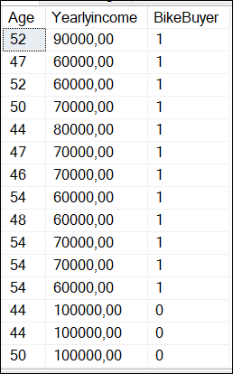
Where BikeBuyer is 1 if the customer is a bike buyer and 0 means that the customer is not a bike buyer.
Finding the number of nodes for K-means
You need to calculate the number of clusters necessary. The following Python code shows how to find the number of clusters required using the elbow method:
import pandas as pd
import pyodbc
from sklearn.cluster import KMeans
import matplotlib.pyplot as plt

# SQL Server Connection to the localhost and the adventureworksdw2019
server = '.'
database = 'AdventureWorksDW2019'

# Windows authentication connection
connection = pyodbc.connect(
f'DRIVER={{SQL Server}};SERVER={server};DATABASE={database};Trusted_Connection=yes;')

# Query to access the vTargetMail view of the Adventureworks2019DW database
Myquery = 'SELECT Age, YearlyIncome, BikeBuyer FROM dbo.vTargetMail'

# Load the data into a Pandas DataFrame and filter for BikeBuyer = 1
df = pd.read_sql(Myquery, connection)
df = df[df['BikeBuyer'] == 1]

# Prepare data for clustering
data = df[['Age', 'YearlyIncome']]
# Find the number of clusters required with the elbow method
inertia_values = []
possible_cluster_values = range(1, 11)
for k in possible_cluster_values:
  km = KMeans(n_clusters=k, random_state=42)

km.fit(data)
inertia_values.append(km.inertia_)

# Plotting the elbow method
plt.plot(possible_cluster_values, inertia_values, marker='o')
plt.xlabel('Number of Clusters')
plt.ylabel('Inertia')
plt.title('Elbow Method to detect the # of Clusters')
plt.show()

# Close your database connection
connection.close()
Explanation of the elbow method
The elbow method is used to calculate the number of clusters. It requires running the K-Means using different values of k and plotting the sum of squared distances (which is called inertia) between data points and their assigned centroids. A centroid is the center point of a cluster. Which is basically the mean position of all the data points in the cluster, and it is used as a central point for that group.
We first invoke the libraries to use:
import pandas as pd
import pyodbc
from sklearn.cluster import KMeans
import matplotlib.pyplot as plt
First, Pyodbc is used to connect to SQL Server to the dbo.vTargetMail view and get the data. Secondly, Pandas will be used to get the data in a Data Frame. Thirdly, Sklearn.cluster is the library for the k-means algorithm and will be used to classify the data in clusters. Finally, the matplotlib is used to graph the data.
Next, we have the connection information:
# SQL Server Connection to the localhost and the adventureworksdw2019
server = '.'
database = 'AdventureWorksDW2019'

# Windows authentication connection
connection = pyodbc.connect(
f'DRIVER={{SQL Server}};SERVER={server};DATABASE={database};Trusted_Connection=yes;')
First, we have the SQL Server name which is the local server which is a “.”. You can also write the SQL Server name. Secondly, we have the database name. In this case, it is the AdventureWorksDW2019. Finally, we use the Windows authentication (trusted_connection=yes) to connect
The next section is doing a query and applying a filter:
# Query to access the vTargetMail view of the Adventureworks2019DW database
Myquery = 'SELECT Age, YearlyIncome, BikeBuyer FROM dbo.vTargetMail'

# Load the data into a Pandas DataFrame and filter for BikeBuyer = 1
df = pd.read_sql(Myquery, connection)
df = df[df['BikeBuyer'] == 1]
Myquery is a simple query to the dbo.vTargetMail view. This view is included in the AdventureworksDW2019 database. We are then applying a filter to analyze only the customer who bought a bike (bikebuyer==1). Also, we will find the required clusters, we will analyze 1 to 11 clusters, and graph them using the K-Means algorithm.
# Find the number of clusters required with the elbow method
inertia_values = []
possible_cluster_values = range(1, 11)

for k in possible_cluster_values:
   km = KMeans(n_clusters=k, random_state=42)

km.fit(data)
inertia_values.append(km.inertia_)
Finally, we will create the chart:
# Plotting the elbow method
plt.plot(possible_cluster_values, inertia_values, marker='o')
plt.xlabel('Number of Clusters')
plt.ylabel('Inertia')
plt.title('Elbow Method to detect the # of Clusters')
plt.show()
The chart created is the following:

As you can see, the inertia is lower after 3 clusters. Then, 3 is the ideal number of clusters.
K-Means applied to SQL Server data
Previously, we found that the ideal number of clusters is 3, after that, the inertia is low. The following code shows how to classify the data in clusters:
import pandas as pd
import pyodbc
from sklearn.cluster import KMeans as km
import matplotlib.pyplot as plt

# SQL Server Connection
server = '.'
database = 'AdventureWorksDW2019'
connection = pyodbc.connect(
f'DRIVER={{SQL Server}};SERVER={server};DATABASE={database};Trusted_Connection=yes;')

# Query to access the vTargetMail view of the Adventureworks2019DW database
Myquery = 'SELECT Age, YearlyIncome, BikeBuyer FROM dbo.vTargetMail'

# Load the data into a Pandas DataFrame and filter for BikeBuyer = 1
df = pd.read_sql(Myquery, connection)
df = df[df['BikeBuyer'] == 1]

# Prepare data for clustering
data = df[['Age', 'YearlyIncome']]

# Apply K-Means using 3 clusters according to the Elbow method
kmeans = km(n_clusters=3, random_state=42)
kmeans.fit(data)

# Scatter plot chart
# add titles, labels x and y
plt.scatter(df['Age'], df['YearlyIncome'], c=kmeans.labels_, cmap='viridis')
plt.xlabel('Age')
plt.ylabel('YearlyIncome')
plt.title('Scatter plot of Age vs YearlyIncome (Clustered)')
plt.show()

# Close your SQL Server database connection
connection.close()
The code is similar to the elbow method. We invoke libraries, connect to the SQL Server view and filter the data where bikeBuyer is 1. Also, we will use 3 clusters based on the elbow method applied previously:
kmeans = km(n_clusters=3, random_state=42)
kmeans.fit(data)
The random_state=42 can be any number. It is an internal seed. The random_state=42 can be any number. It is an internal seed.
Analyzing K-Means applied to SQL Server data
The chart generated by the Python code is the following:

First, we have the yellow cluster with a yearly income from 0 to 40000. These customers buy the bikes until they are 80 years old. After that, they do not buy too much.
Secondly, we have the cluster from 50000 until 90000. The customers that earn 5000 are regular customers until they are 55 years old. After that age, the number of customers is lower. From 60000 until 90000 the customers are regular until 80-85 years old.
Finally, the last cluster is customers with a yearly income from 100000 to 170000. This group is special. For example, there are no customers with a salary of 140000. These customers are irregular users when they are 65 years old.
Conclusion
In this article, we used the K-Means algorithm to classify the data in clusters. First, we used the Elbow method to determine the number of clusters and then we created the code to divide the data using 3 clusters. K-means is a nice algorithm used to analyze data. You can find nice patterns with this algorithm that in many cases the human cannot detect.
Images
Some images were created in Bing.
The post Machine learning K-Means applied to SQL Server data appeared first on SQLServerCentral.
]]>The post SQL Server and Python Tutorial appeared first on SQLServerCentral.
]]>In this article, we will see how to connect SQL Server with Python using the pyodbc library. If you are a SQL DBA, we strongly recommend running Python scripts in SSMS.
However, we have some Python developers who want to work with Python directly instead of working with SSMS and enabling scripts. We will cover the following topics:
- First, we will see how to connect SQL Server with Python and get data using pyodbc.
- Secondly, we will get data from SQL Server using a stored procedure with Python.
- Thirdly, we will insert data to SQL Server using a stored procedure in Python.
- Finally, we will insert data from a CSV file into SQL Server.
Requirements
- First, you will need SQL Server database engine installed.
- Secondly, a Python Code Editor. In my case, I will use the Visual Studio Code, but you can use any software of your preference.
- Thirdly, the Adventureworks2019 database. You can use a different database, but you will need to modify the code.
- Finally, and optionally, I recommend installing SQL Server Management Studio to verify the data.
How to connect SQL Server with Python and get data using pyodbc
The following code will connect to SQL Server and get information from the person.person table.
import pyodbc

#Connection information
# Your SQL Server instance
sqlServerName = '.'

#Your database
databaseName = 'AdventureWorks2019'

# Use Windows authentication
trusted_connection = 'yes'

# Connection string information
connenction_string = (
f"DRIVER={{SQL Server}};"
f"SERVER={sqlServerName};"
f"DATABASE={databaseName};"
f"Trusted_Connection={trusted_connection}"
)

try:
   # Create a connection
   connection = pyodbc.connect(connenction_string )
   cursor = connection.cursor()
   # Run the query to the Person.Person table
   query = 'SELECT * FROM Person.Person'
   cursor.execute(query)

   # print the results of the row
   rows = cursor.fetchall()

   for row in rows:
      print(row)
except pyodbc.Error as ex:
      print("An error occurred in SQL Server:", ex)

# Close the connection
finally:
First, we use the import pyodbc library. If you do not have this library installed in the command line, you need to install the pyodbc for Python:
pip install pyodbc
The next lines will connect to the local SQL Server, the Adventureworks2019 database using Windows Authentication:
#Connection information
# Your SQL Server instance
sqlServerName = '.'

#Your database
databaseName = 'AdventureWorks2019'

# Use Windows authentication
trusted_connection = 'yes'

# Connection string information
connenction_string = (
f"DRIVER={{SQL Server}};"
f"SERVER={sqlServerName};"
f"DATABASE={databaseName};"
Next, we use the connection and run the query. The query will get the data from the Person.Person table of the Adventureworks2019 database.
# Create a connection
connection = pyodbc.connect(connenction_string )
cursor = connection.cursor()

# Run the query to the Person.Person table
query = 'SELECT * FROM Person.Person'

cursor.execute(query)
Finally, we print the results and close the connection.
except pyodbc.Error as ex:
   print("An error occurred in SQL Server:", ex)

# Close the connection
finally:
   if 'connection' in locals():
       connection.close()
Get data from SQL Server using a stored procedure with Python
Now, we will create the code to connect to SQL Server invoking a SQL Server Stored Procedure in Python.
First, we will create the stored procedure code to get the information from the person.person table.
CREATE PROCEDURE [dbo].[GetPersons]
AS
SELECT * FROM Person.Person;
Secondly, we will invoke the stored procedure created using Python:
import pyodbc

# Connection information

sqlServerName = '.' # Your SQL Server instance

databaseName = 'AdventureWorks2019'

trusted_connection = 'yes' # Use Windows authentication

# Connection string information

connection_string = (

f"DRIVER={{SQL Server}};"

f"SERVER={sqlServerName};"

f"DATABASE={databaseName};"

f"Trusted_Connection={trusted_connection}"

)

try:

# Create a connection

connection = pyodbc.connect(connection_string)

cursor = connection.cursor()

# Execute the stored procedure

stored_procedure = 'GetPersons'

# Call the stored procedure

cursor.execute("{CALL " + stored_procedure + "}")

# Fetch and print the results

rows = cursor.fetchall()

for row in rows:

print(row)

except pyodbc.Error as ex:

print("An error occurred in SQL Server:", ex)

finally:

# Close the connection

if 'connection' in locals():

connection.close()

Most of the lines are similar that the first example running a query.
Most of the lines are similar to the first example running a query.
Here are the lines of code that are different:
stored_procedure = 'GetPersons'

# Call the stored procedure

cursor.execute("{CALL " + stored_procedure + "}")
We are invoking the stored procedure GetPersons.
Insert data to SQL Server using a stored procedure in Python
In the next example, we will create a stored procedure that inserts data into a SQL Server database.
First, we will create a stored procedure with parameters to insert data into the sales.currency table:
CREATE PROCEDURE [dbo].[InsertCurrency]
  @CurrencyCode nchar(3),
  @Name dbo.Name
AS
INSERT INTO [Sales].[Currency] ([CurrencyCode], [Name], [ModifiedDate])
 VALUES (@CurrencyCode, @Name, GETDATE());
Secondly, we will create the Python code to invoke the stored procedure:
import pyodbc

# Connection information
sqlServerName = '.' # Your SQL Server instance
databaseName = 'AdventureWorks2019'
trusted_connection = 'yes' # Use Windows authentication

# Connection string information
connection_string = (
 f"DRIVER={{SQL Server}};"
 f"SERVER={sqlServerName};"
 f"DATABASE={databaseName};"
 f"Trusted_Connection={trusted_connection}"
 )

try:
    # Create a connection
    connection = pyodbc.connect(connection_string)

    cursor = connection.cursor()

    # Parameters used by the stored procedure
    currency_code = 'MEU'

    name = 'Sql Server Central Euros'

    # Call the stored procedure
    stored_procedure = 'InsertCurrency'

    cursor.execute("{CALL " + stored_procedure + " (?, ?)}", (currency_code, name))

    # Commit the transaction
    connection.commit()

    print("Stored procedure executed successfully!")
except pyodbc.Error as ex:
    print("An error occurred in SQL Server:", ex)
    connection.rollback()
finally:
    # Close the connection
    if 'connection' in locals():
        connection.close()
If everything is OK, the Python code will insert data into the sales.currency table.
The following lines are the most important ones:
# Parameters used by the stored procedure

currency_code = 'MEU'

name = 'Sql Server Central Euros'

# Call the stored procedure

stored_procedure = 'InsertCurrency'

cursor.execute("{CALL " + stored_procedure + " (?, ?)}", (currency_code, name))
Basically, we will insert the currency code and a name for the currency. Then we invoke the stored procedure and send values to 2 parameters.
If everything is OK, we will see the new data inserted:

Insert data from a CSV file into SQL Server
Finally, we have this CSV file named currencies.csv with this data:
WIZ, Wizarding Galleon
STK, Starkmark
FOR, Jedi Credit
AVC, Avenger Coin
NRN, Narnian Silver Star
PTW, Galleon of Wizardry
MTR, Neo Coin
WAK, Wakandan Vibranium Token
We want to insert the data from the csv file into the sales.currency table. The following Python code will do that:
import pyodbc
import csv

# Connection information
sqlServerName = '.' # Your SQL Server name
databaseName = 'AdventureWorks2019'
trusted_connection = 'yes' # Use Windows authentication

# Connection string information
connection_string = (
f"DRIVER={{SQL Server}};"
f"SERVER={sqlServerName};"
f"DATABASE={databaseName};"
f"Trusted_Connection={trusted_connection}"
)

try:
    # Create a connection
    connection = pyodbc.connect(connection_string)

    cursor = connection.cursor()

    # Read currencies from CSV file and insert into the database
    with open('c:\data\currencies.csv', 'r') as csv_file:
        csv_reader = csv.reader(csv_file)
        next(csv_reader) # Skip the header row if it exists
        for row in csv_reader:
             currency_code = row[0]
             name = row[1]

        stored_procedure = 'InsertCurrency'
        cursor.execute("{CALL " + stored_procedure + " (?, ?)}", (currency_code, name))

        connection.commit()
        print(f"Inserted: {currency_code}, {name}")
        print("All currencies inserted successfully!")
except pyodbc.Error as ex:
    print("An error occurred in SQL Server:", ex)
    connection.rollback()
finally:
    # Close the connection
    if 'connection' in locals():
        connection.close()
First, we read the data from the csv file.
# Read currencies from CSV file and insert into the database

with open('c:\data\currencies.csv', 'r') as csv_file:

csv_reader = csv.reader(csv_file)

next(csv_reader)
Secondly, we read the values in rows.
for row in csv_reader:

currency_code = row[0]

name = row[1]
Finally, we execute the stored procedure and insert the values.
stored_procedure = 'InsertCurrency'

cursor.execute("{CALL " + stored_procedure + " (?, ?)}", (currency_code, name))
Conclusion
In this article, we learned how to connect to SQL Server using the pyodbc. We learned how to run a query, how to run stored procedures with parameters, and finally, we imported data from a csv file into SQL Server using Python.
Images
Some images were generated in Bing Image Creator.
The post SQL Server and Python Tutorial appeared first on SQLServerCentral.
]]>The post Integrating Python with MongoDB appeared first on SQLServerCentral.
]]>MongoDB has gained significant popularity as a NoSQL database solution due to its flexibility, scalability, and document-oriented nature. Python, on the other hand, is a versatile programming language known for its ease of use and rich ecosystem of libraries. This article explores the integration of Python with MongoDB, covering fundamental concepts with practical implementation steps using the pymongo library. The integration of these two technologies provides developers with a powerful toolset for building modern and efficient applications.
Overview of MongoDB
MongoDB is a popular NoSQL database that offers a flexible, document-oriented approach to data storage. Unlike traditional relational databases, which store data in tables, MongoDB stores data in collections of JSON-like documents. This allows developers to store and retrieve complex, unstructured, or semi-structured data more efficiently. Some of the key features of MongoDB are:
- Document-Oriented: MongoDB stores data in documents, which are self-contained units that can hold various types of data without requiring a fixed schema.
- Scalability: MongoDB supports horizontal scaling by distributing data across multiple servers, making it suitable for handling large datasets and high traffic.
- Flexibility: The dynamic schema of MongoDB enables changes to the data structure without affecting existing records, making it adaptable to evolving application needs.
- Indexes: MongoDB supports various index types, enabling efficient data retrieval and improving query performance.
- Query Language: MongoDB's query language allows you to filter, sort, and transform data using JSON-like queries.
- Aggregation Framework: The aggregation framework provides powerful tools for data transformation, analysis, and reporting.
- Geospatial Capabilities: MongoDB offers geospatial indexing and querying to handle location-based data.
- Replication and High Availability: MongoDB supports replica sets to provide data redundancy and automatic failover in case of server failures.
- Security: MongoDB offers authentication, authorization, and role-based access control to ensure data security.
Integrating Python with MongoDB using pymongo Library
Let's go through a simple example of how to integrate Python with MongoDB using the pymongo library which provides a Python API for working with MongoDB databases. In this example, we'll cover the process of connecting to a MongoDB database, reading data, inserting data, querying data, and updating data.
You can use MongoDB version 3.6 or later and Python version 3.6 or later to carry out the steps below.
Step 1: Install the pymongo Library
First, you need to install the pymongo library if you haven't already. You can install it using pip:
pip install pymongo
Step 2: Import the Required Modules
In your Python script, import the pymongo module to use its functionalities:
import pymongo
Step 3: Connect to MongoDB
To connect to a MongoDB server, you need to create a MongoClient object. Provide the appropriate MongoDB connection URL as an argument. This URL typically includes information about the server's address, port, and authentication credentials.
# Replace 'your_connection_url' with your actual MongoDB connection URL
client = pymongo.MongoClient('your_connection_url')
Here’s a sample:
from pymongo import MongoClient

client = MongoClient('localhost', 27017)
Step 4: Access Databases and Collections
Once connected, you can access a specific database and collection within that database. In this example, we'll use a database named "testdb" and a collection named "example_collection".
# Access the 'testdb' database
db = client['testdb']

# Access the 'example_collection' collection
collection = db['example_collection']
Step 5: Insert Data into the Collection
You can insert documents (data) into the collection using the insert_one() or insert_many() methods.
Here, we'll insert a single document using insert_one() method. The insert_one() method is a function provided by the pymongo library in Python, which is used to insert a single document (also referred to as a record or data item) into a MongoDB collection. It's a common operation when working with databases to add new data to a collection.
# Prepare a document to insert
document = {
    'name': 'John Doe',
    'age': 30,
    'email': '[email protected]'
}

# Insert the document into the collection
insert_result = collection.insert_one(document)

# Print the inserted document's ObjectId
print(f"Inserted document ID: {insert_result.inserted_id}")
Step 6: Query Data from the Collection
You can use find() method to query data from a MongoDB collection. It allows you to retrieve documents (data items) that match a specific query criteria. The find() method returns a cursor, which is an iterable object that you can use to access the matching documents.
# Query for documents with age greater than 25
query = {'age': {'$gt': 25}}
results = collection.find(query)

# Print the matching documents
for result in results:
    print(result)
Step 7: Update Data in the Collection
To update data, use the update_one() or update_many() methods. Here, we'll update a single document using update_one() method. The update_one() method is a function provided by the pymongo library in Python, used to update a single document within a MongoDB collection. It allows you to modify specific fields or attributes of a document that matches a given query. The update_one() method is useful when you want to change specific data without affecting multiple documents.
# Update the email address of a document
update_query = {'name': 'John Doe'}
update_data = {'$set': {'email': '[email protected]'}}
update_result = collection.update_one(update_query, update_data)

# Print the number of documents updated
print(f"Documents updated: {update_result.modified_count}")
Step 8: Delete Data in the Collection
You can delete data using the delete_one() and delete_many() methods. Here, we'll delete a single document. Just like update_one(), this method allows you to remove a specific data item from the collection without affecting multiple documents.
# Delete a document with a specific name
delete_query = {'name': 'John Doe'}
delete_result = collection.delete_one(delete_query)

# Print the number of documents deleted
print(f"Documents deleted: {delete_result.deleted_count}")
Step 9: Disconnect from MongoDB
After performing your operations, close the connection to the MongoDB server:
# Close the MongoDB connection
client.close()
Conclusion
In the above example, we imported the pymongo module and established a connection to the MongoDB server using the MongoClient class. We accessed a specific database and collection using dictionary-style access. We inserted a document using the insert_one() method and printed the inserted document's ObjectId. We queried data using the find() method and printed the matching documents. We updated a document using the update_one() method and printed the number of modified documents. We deleted a document using the delete_one() method and printed the number of deleted documents. Finally, we closed the connection to the MongoDB server.
Remember that MongoDB provides a flexible schema, meaning different documents within the same collection can have varying structures. The pymongo library automatically handles the conversion between Python data structures and BSON (Binary JSON), which is the format used by MongoDB.
By integrating Python with MongoDB using the pymongo library, you can leverage MongoDB's flexibility and scalability to efficiently manage and manipulate data in your applications.
The post Integrating Python with MongoDB appeared first on SQLServerCentral.
]]>The post Sentiment Analysis with AI appeared first on SQLServerCentral.
]]>In this article, we will do sentiment analysis of text stored in SQL Server with comments about a product, read the text with AI, and detect customer sentiments. We do this by reading text and then using AI to detect the tone of the text.

In other words, we will do a sentiment analysis of data stored in SQL Server. Read the text and detect if the customer is happy or unhappy with the products and then create a report of the data.
Requirements for the sentiment analysis
- First, you will need SQL Server installed.
- Secondly, a database created in SQL Server. In this example I am using Adventureworks2019, however, any database can be used because we will create new tables from scratch.
- Thirdly, you need a code editor to create Python code. I am using Visual Studio Code, but you can use Visual Studio, Jupiter Notebook, Notepad++, or any other code editor you prefer.
- Optionally, you can install SQL Server Management Studio. It is not mandatory, but it is my favorite tool to handle T-SQL code.
Getting started with Sentiment analysis with AI
Using your code editor write the following code:
from textblob import TextBlob

# Comment
comment = "I hate this product"

# Create an object
obj = TextBlob(comment)

# detect sentiment
sentiment = obj.sentiment

# Get polarity
polarity = sentiment.polarity

# Print polarity and subjetivity
print("Polarity:", polarity)
First, you will need the textblob library. This library is a nice API used for NLP (Natural Language Processing). The library is used for speech tagging, phrase extraction, translation, and in our case sentiment analysis. If it is not installed by default, you will need to go to the command line and run this code where Python is installed:
pip install textbblob
Also, you will need to import the library:
from textblob import TextBlob
In addition, we have the comment. It contains the text that we want to analyze. We will store it in the comment variable.
# Comment
comment = "I hate this product"
Additionally, we create the object and detect the sentiment:
# Create an object
obj = TextBlob(comment)

# detect sentiment
sentiment = obj.sentiment
Finally, we get the polarity and print the results.
polarity = sentiment.polarity

# Print polarity and subjetivity
print("Polarity:", polarity)
Sentiment analysis and the polarity
The polarity is the measure used to analyze the sentiments related to the text. Our library reads the text and detects if the customer is happy or not. The following table shows examples of possible values and their explanations:
| Polarity | Sentiment Explanation |
| -1.0 | Strongly negative sentiment indicating extreme dislike or hatred. |
| -0.9 | Very negative sentiment expressing strong dissatisfaction. |
| -0.8 | Highly negative sentiment indicating strong disapproval. |
| -0.7 | Negative sentiment conveying significant dislike. |
| -0.6 | Moderately negative sentiment expressing dissatisfaction. |
| -0.5 | Mildly negative sentiment indicating slight disappointment. |
| -0.4 | Slightly negative sentiment suggesting some criticism. |
| -0.3 | Slightly negative sentiment conveying minor dissatisfaction. |
| -0.2 | Slight negativity with a hint of dissatisfaction. |
| -0.1 | Slight negativity with a touch of criticism. |
| 0.0 | Neutral sentiment with no clear positive or negative opinion. |
| 0.1 | Slight positivity with a hint of approval. |
| 0.2 | Slight positivity suggests mild satisfaction. |
| 0.3 | Slightly positive sentiment conveying some appreciation. |
| 0.4 | Mildly positive sentiment indicates moderate approval. |
| 0.5 | Positive sentiment expressing satisfaction. |
| 0.6 | Moderately positive sentiment conveying significant approval. |
| 0.7 | Highly positive sentiment indicating strong approval. |
| 0.8 | Very positive sentiment expressing intense satisfaction. |
| 0.9 | Extremely positive sentiment conveying extreme admiration. |
| 1.0 | Strongly positive sentiment suggesting intense love or adoration. |
If we run the code, the value of the comment “I hate this product” will show the following value:
Polarity: -0.8
The text has a highly negative sentiment.
If we modify the comment line with a positive value, the polarity will change:
# Comment

comment = "I liked the product. It was useful to me. Thanks."
If we run the code, the polarity is the following:
Polarity: 0.36666666666666664
This value is a Mildly positive sentiment.
Sentiment Analysis with SQL Server
Previously, we try to work with Python directly. Now we have several sentiments stored in our SQL Server database. How can we detect the sentiment of several users using our data stored in SQL Server?
First, we will create a table for this example:
CREATE TABLE sentiments (
id INT IDENTITY(1,1) PRIMARY KEY,
comment VARCHAR(MAX),
sentiment DECIMAL(4,2)
);
Where id is an identity column and the numbers are generated automatically. The comment will store the comments and the sentiments will be detected later.
Secondly, we will insert some comments:
INSERT INTO sentiments (comment)
VALUES
('This software is amazing! It has greatly improved our productivity.'),
('I''m really impressed with the features and functionality of this software.'),
('The user interface is intuitive and easy to navigate.'),
('I encountered several bugs while using this software. Needs improvement.'),
('The customer support for this software is top-notch.'),
('I find the performance of this software to be quite slow.'),
('The latest update of this software introduced new useful features.'),
('I''m disappointed with the lack of documentation for this software.'),
('The software crashes frequently, making it unreliable.'),
('The pricing of this software is reasonable considering its features.'),
('The user experience of this software needs a lot of improvement.'),
('I love how customizable this software is to suit our needs.'),
('The installation process of this software was a breeze.'),
('I encountered compatibility issues with other software while using this.'),
('The software''s interface is outdated and needs a modern look.'),
('This software has become an essential tool in our daily operations.'),
('I''m frustrated with the frequent updates that disrupt our workflow.'),
('The software lacks important functionalities that we require.'),
('The user interface could be more intuitive and user-friendly.'),
('I appreciate the regular updates and bug fixes for this software.');
Finally, we will create the Python code to detect and insert the sentiment value into the sentiment column of the sentiments SQL Server table.
Python code for Sentiment Analysis in SQL Server
The following code will read the sentiment assign a polarity value and update the values in the SQL Server table:
import pyodbc

from textblob import TextBlob

# Connect to the SQL Server database
conn = pyodbc.connect('Driver={SQL Server};'
'Server=.;'
'Database=adventureworks2019;'
'Trusted_Connection=yes;')

# Retrieve the comments from the SQL Server database
cursor = conn.cursor()
cursor.execute("SELECT id, comment FROM sentiments;")
rows = cursor.fetchall()

# Iterate over the rows and update the sentiment column
for row in rows:
   comment_id = row.id
   comment_text = row.comment

   # Create a TextBlob object for the comment
   obj = TextBlob(comment_text)

   # Detect sentiment
   sentiment = obj.sentiment

   # Get polarity
   polarity = sentiment.polarity

   # Update the sentiment column in the database
   update_cursor = conn.cursor()
   update_cursor.execute("UPDATE sentiments SET sentiment = ? WHERE id = ?;", polarity, comment_id)
   update_cursor.commit()

# Close the cursors and connection
cursor.close()
conn.close()
The code will connect to SQL Server. If you do not have the pyodbc library installed, you may need to install the pyodbc in Python using the command line (pip install pyodbc). Once installed, the following code can be used.
# Connect to the SQL Server database
conn = pyodbc.connect('Driver={SQL Server};'
'Server=.;'
'Database=adventureworks2019;'
'Trusted_Connection=yes;')
The server is the SQL Server name. In this case. means to use the local SQL Server. Otherwise, write the name of the SQL Server. The database contains the database name where the table sentiments are stored. If your table was created in a different database, change the name accordingly. Finally, trusted connection means connecting to SQL Server using Windows Authentication.
Also, we will retrieve the comments from the sentiments table using a cursor.
# Retrieve the comments from the SQL Server database
cursor = conn.cursor()
cursor.execute("SELECT id, comment FROM sentiments;")
rows = cursor.fetchall()
In addition, we will iterate the values of the rows and store the comments and comment id. Next, we will create the object and detect the sentiment as in the previous example.
# Iterate over the rows and update the sentiment column
for row in rows:
   comment_id = row.id
   comment_text = row.comment
   # Create a TextBlob object for the comment
   obj = TextBlob(comment_text)
   # Detect sentiment
   sentiment = obj.sentiment
Additionally, we will detect the polarity and update the sentiments table and the sentiment column with the polarity detected in each row.
# Get polarity
polarity = sentiment.polarity

# Update the sentiment column in the database
update_cursor = conn.cursor()
update_cursor.execute("UPDATE sentiments SET sentiment = ? WHERE id = ?;", polarity, comment_id)
update_cursor.commit()
Finally, we will close the cursor and the connection.
# Close the cursors and connection
cursor.close()
conn.close()
Sentiment analysis in SQL Server – check final results
Previously, we detected the polarity in the sentiments table. In order to verify the results, we will do a select of the data:
SELECT *
FROM sentiments
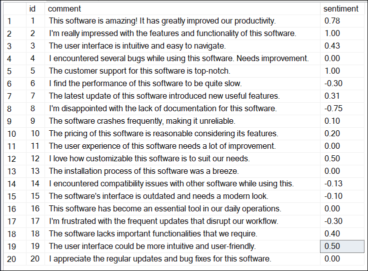
Also, we will count the negative sentiments, positive and neutral (0). Finally, we will check the average sentiment.
SELECT
  AVG(sentiment) AS average_sentiment,
  COUNT(CASE WHEN sentiment < 0 THEN 1 END) AS negative_sentiments,
  COUNT(CASE WHEN sentiment = 0 THEN 1 END) AS neutral_sentiments,
  COUNT(CASE WHEN sentiment > 0 THEN 1 END) AS positive_sentiments
 FROM Sentiments

The sentiments are slightly positive in general with a value of 0.18. It is not so positive in general, but at least it is positive. In addition, there are 5/20 negative sentiments and 5/20 neutral sentiments, and 10/20 positive sentiments. There are more positive sentiments in general.
Finally, let’s check the positive/neutral/negative sentiments in percentage.
SELECT
  AVG (sentiment) AS average_sentiment
, COUNT (CASE
           WHEN sentiment < 0 THEN
             1
         END) * 100.0 / COUNT (*) AS negative_sentiments_percentage
, COUNT (CASE
           WHEN sentiment = 0 THEN
             1
         END) * 100.0 / COUNT (*) AS neutral_sentiments_percentage
, COUNT (CASE
           WHEN sentiment > 0 THEN
             1
         END) * 100.0 / COUNT (*) AS positive_sentiments_percentage
FROM Sentiments;
The code shows the positive/neutral/negative sentiments in percentage. The negative sentiments are 25 %, neutral sentiments 25 %, and positive sentiments 50 %.

Conclusion
In this article, we learn how to do sentiment analysis in Python. Also, we learned how to detect the sentiments of comments in an SQL Server table using Python. Finally, we detect some statistics using T-SQL code to analyze the sentiments in general.
The post Sentiment Analysis with AI appeared first on SQLServerCentral.
]]>Screen scraping enables developers to create solutions that permit comparative analyses from all over the internet, such as web applications that look for the best price on an item from many different online stores.
The post Screen Scraping with Python and BeautifulSoup Code Examples appeared first on SQLServerCentral.
]]>The post Modifying MySQL data from within Python appeared first on SQLServerCentral.
]]>The post Modifying MySQL data from within Python appeared first on SQLServerCentral.
]]>