Prediction of Bike Sharing Demand using python

• Kaggle: https://www.kaggle.com/c/bike-sharing-demand
• Dataset: https://archive.ics.uci.edu/ml/datasets/Bike+Sharing+Dataset

• Predicted the demand feature using the multiple linear regression model.
• Removed irrelevant features using Exploratory Data Analysis and Correlation matrix.
• Solved the problem of Auto-correlation among the data points. Considered top 3 correlations.
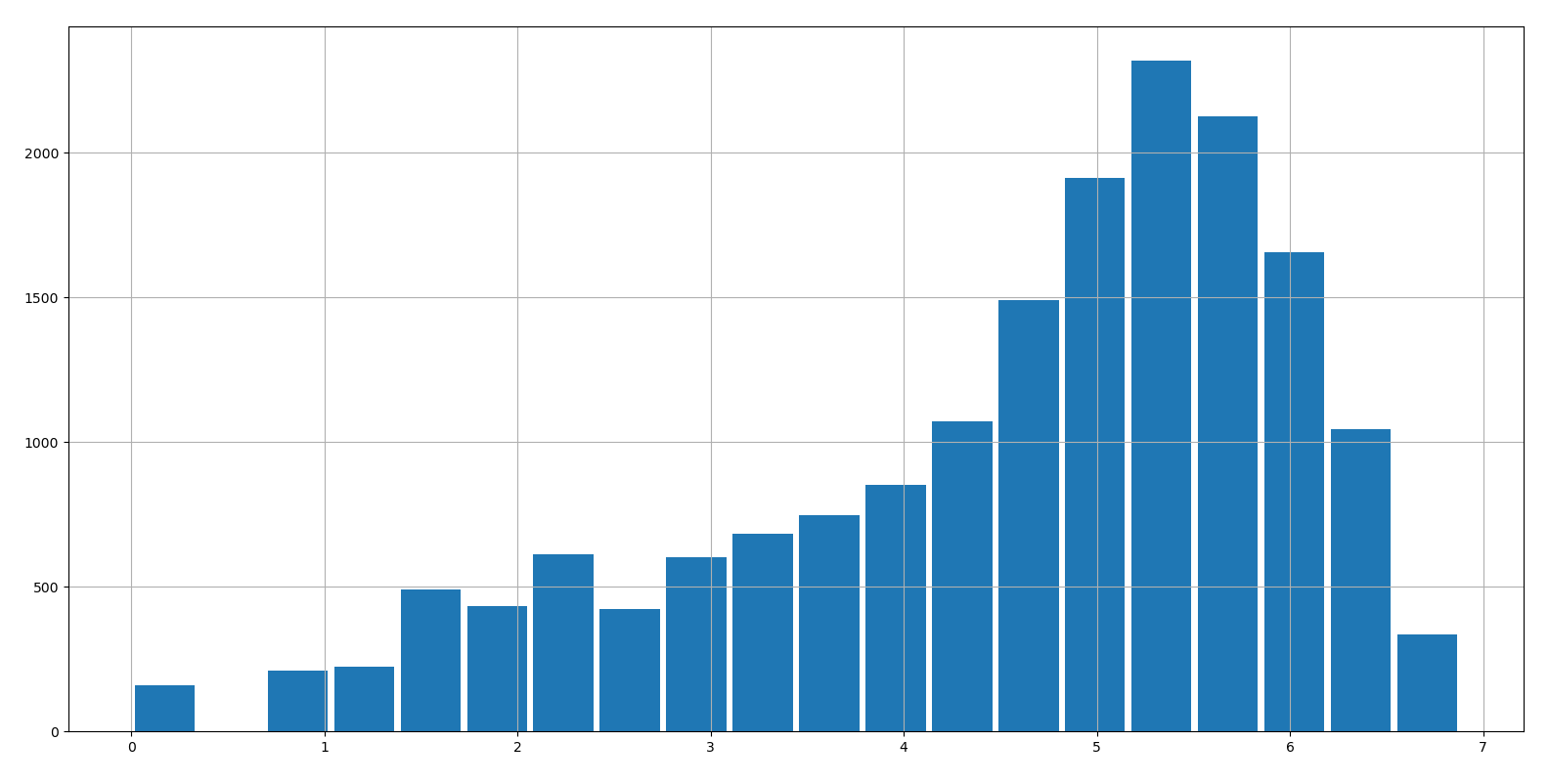
• Solved the problem of Non-Normality of demand feature. Demand was log-normally distributed.
• Successfully calculated the RMSLE score of 0.356

1. date
2. season - (1:winter, 2:spring, 3:summer, 4:fall)
3. year
4. month - (1:12)
5. hour
6. holiday - 1: Yes, 0: No
7. weekday - 0-6 (Sunday to Saturday)
8. workingday - 1: Yes, 0: No
9. weather - 1: Clear, 2: Mist, 3: Light rain/Light Snow, 4: Heavy rain + Ice pallets
10. temp - Normalized temperature in celsius
11. atemp - Normalized feeling temperature in celsius
12. humidity
13. windspeed
14. casual
15. registered
16. demand

• Step 1 - Import the libraries
• Step 2 - Read the CSV file
• Step 3 - Prelim Analysis and Feature Selection
• Step 4 - Data Visualization
• Step 5 - Check for Outliers
• Step 6 - Check for multiple linear regression assumptions
• Step 7 - Create/modify the variables and solving the problem of normality
• Step 8 - Solving the problem of autocorrelation
• Step 9 - Create the dummy variables and drop first to avoid dummy variable trap using get dummies
• Step 9 - Create Test and Train split
• Step 10 - Create the model. Fit and score the model
• Final step - Calculate RMSLE and compare results

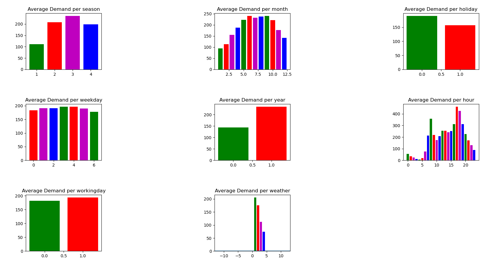
Data visualization Analysis results of Categorical Features

1. There is variation in demand based on
1. Season - Highest demand in Fall season and Lowest demand in Spring season
2. Month - High demand from May to October
3. Holiday - Demand is less on holidays
4. Hour - Peak demand at 8am and 5pm
5. Weather - Highest demand in clear weather and Lowest demand in heavy rainy weather
2. No significant change in demand due to weekday or working day
3. Year-wise growth pattern not considered due to limited number of years

Features to drop

1. Weekdays
2. Year
3. Working day

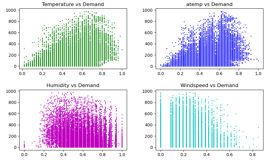
Data visualization Analysis results of Continuous Features

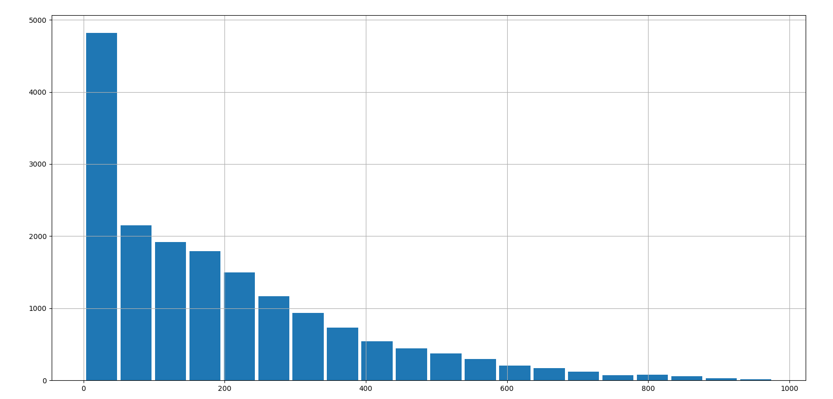
• Predicted variable 'demand' is not normally distributed
• Temperature and demand appears to have direct correlation
• The plot for temp and atemp appear almost identical
• Humidity and windspeed need more statistical analysis

Features to drop

1. atemp
2. windspeed